Data Wrangling Part 1 - Basics of Data Processing
This note is the first part of the “Data Wrangling” trial tour, “Basics of Data Processing,” designed to help you efficiently experience Exploratory’s data wrangling (processing and formatting) functions through hands-on practice.
We hope you’ll experience the convenient features for general data processing when wrangling data in Exploratory.
The estimated time required is about 20 minutes.
Let’s get started!
Creating a Project
In Exploratory, all data analysis, including data import, is done within projects.
Therefore, you first need to create a base project.
Click the “Create New” button from the project management screen.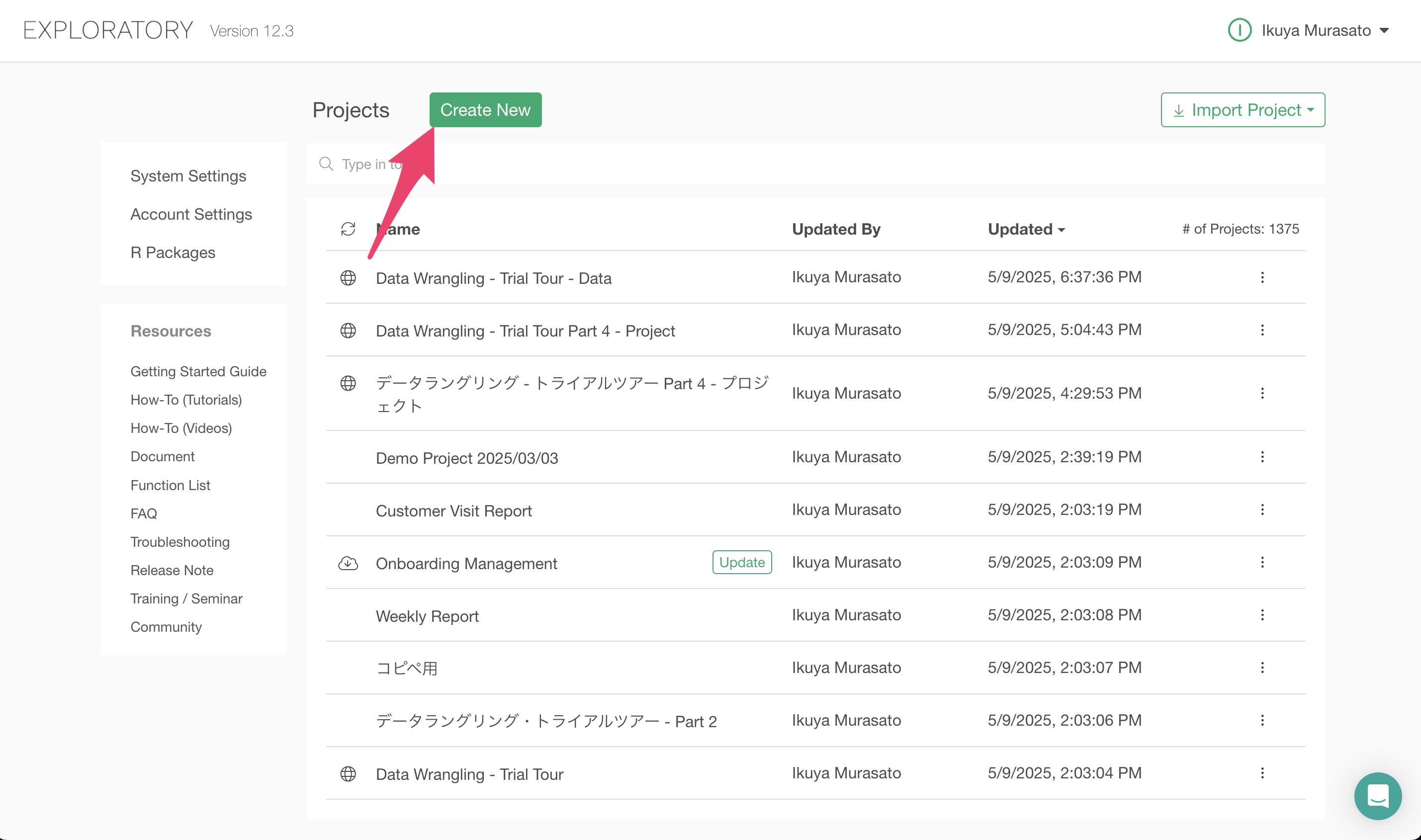
For details on how to create a project, please refer to here.
Importing Data
Once you’ve created a project, let’s import data.
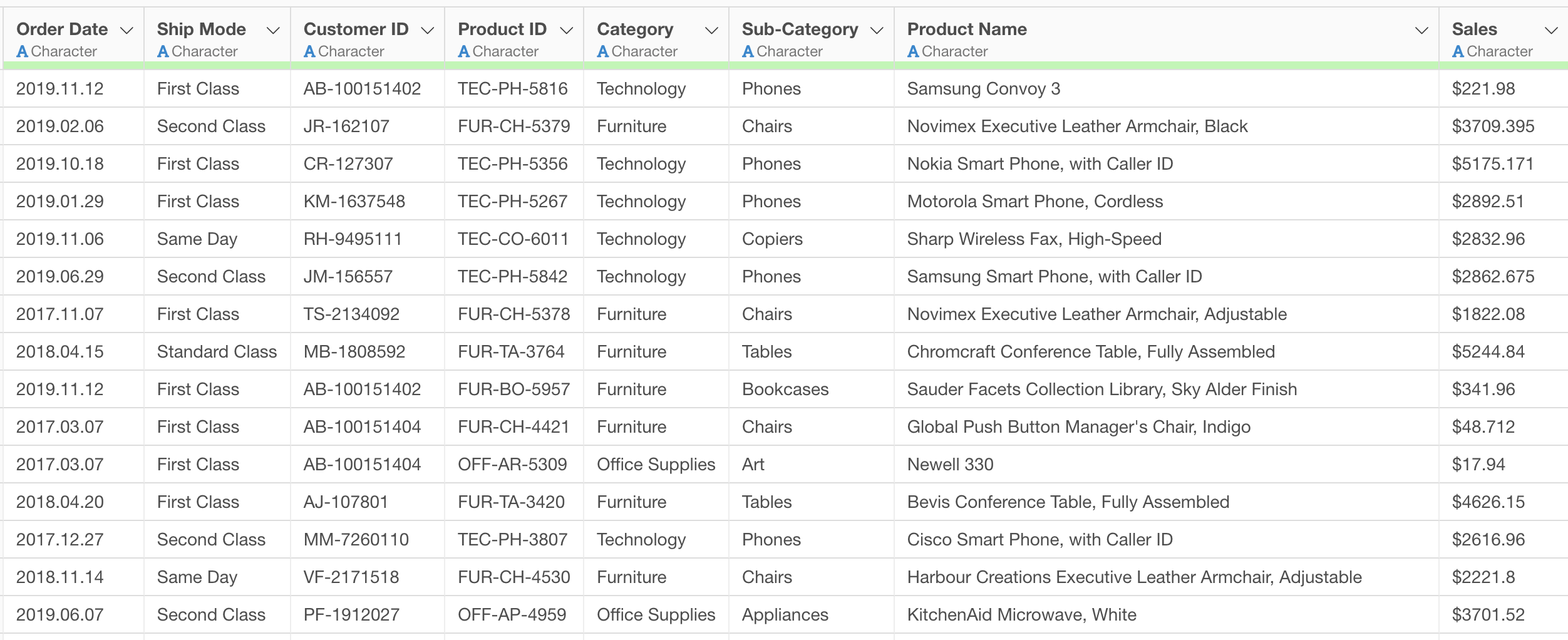
We’ll use “sales” data as our sample data. This data has one row per order (strictly speaking, per line item), with columns for order information such as order date, product category ordered, sales, etc.
You can download the data from this page.
Once you’ve downloaded the CSV file, import it into Exploratory Desktop. No special settings are needed when importing this data, but for details on how to import CSV data, please refer to here.
From here, we’ll use the imported sales data to actually process the data.
Processing Data with AI Prompt
In this section, you’ll experience AI Prompt, but if you want to know more details about AI Prompt, please refer to this link.
Let’s process data using AI Prompt.
1. Converting Data Types
In data analysis, it’s very important that each column is set with the appropriate data type.
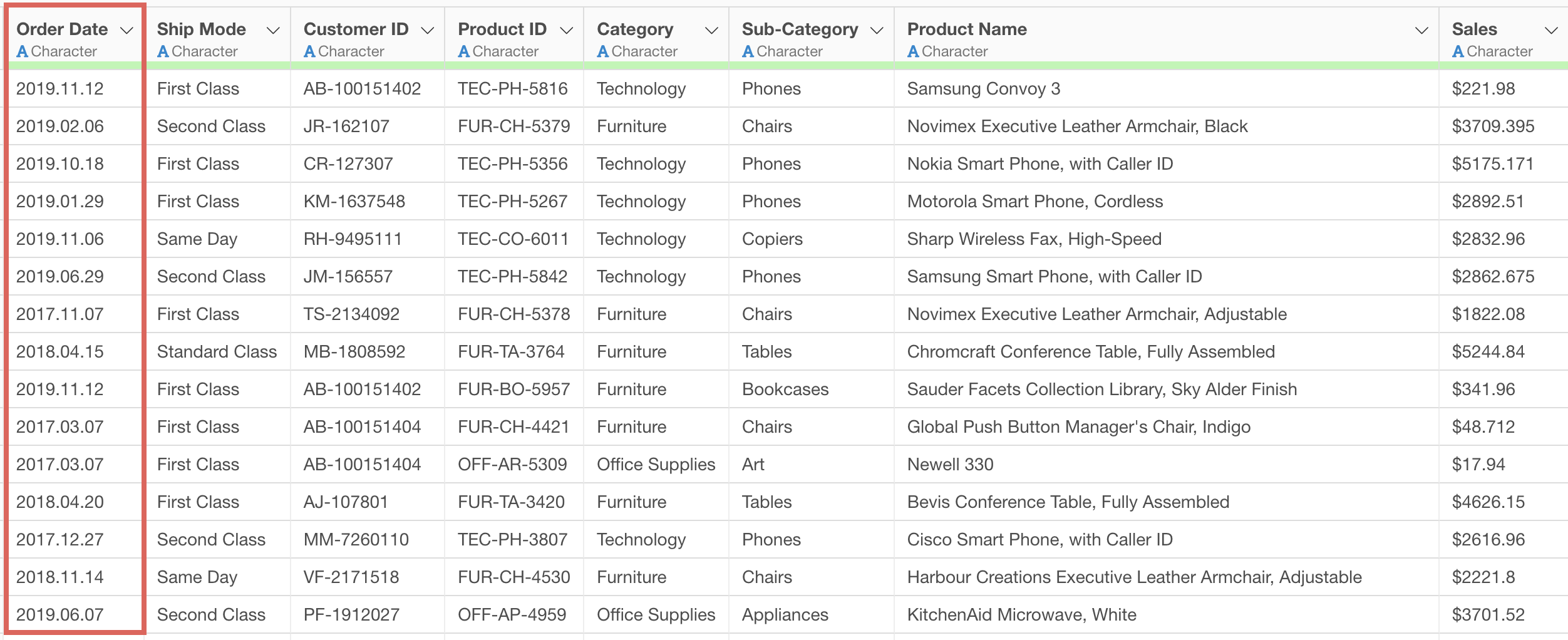
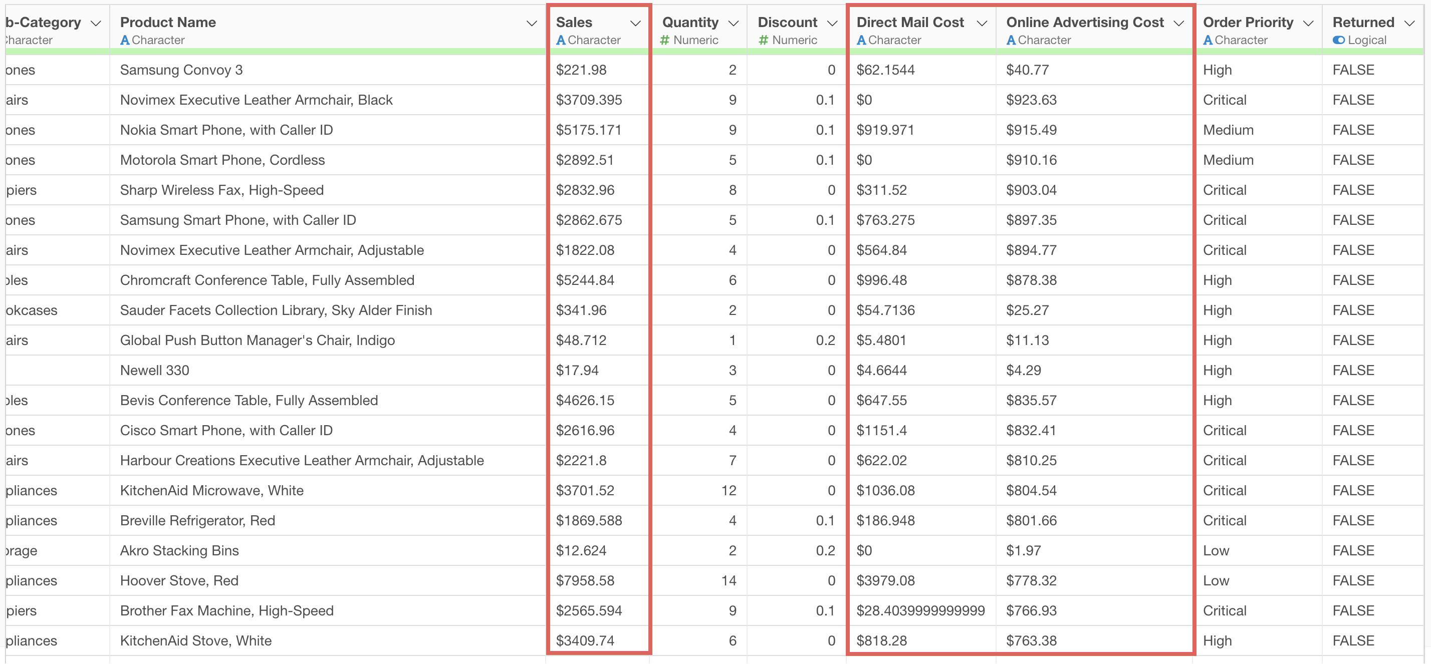
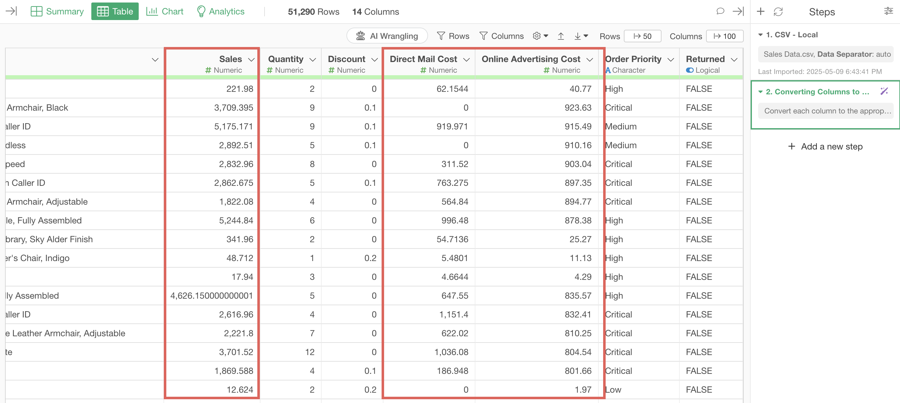
Looking at the current dataframe, we can see that “Order Date” is a string type.
Also, the “Sales,” “Direct Mail Cost,” and “Online Ad Cost” columns contain characters ($) within the numbers, so they are string types.
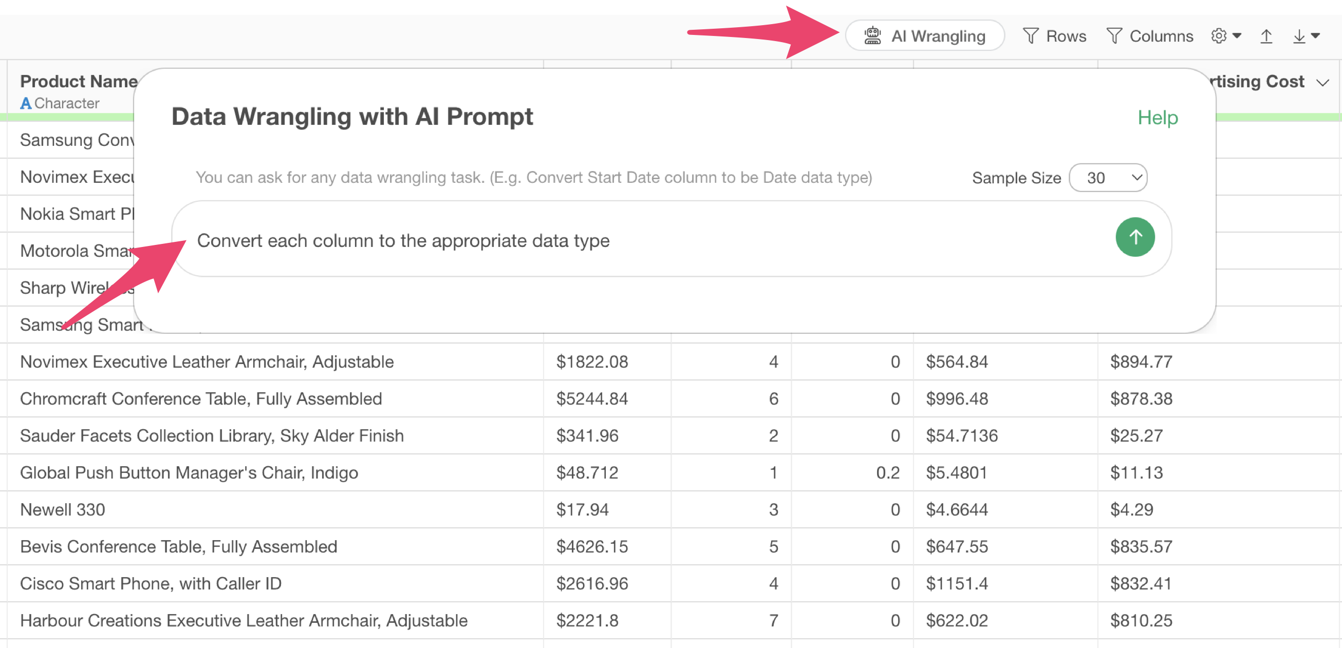
To convert these to appropriate data types, click the “AI Wrangling” button, and when the AI Prompt dialog appears, enter the following text and execute:
Convert each column to the appropriate data type
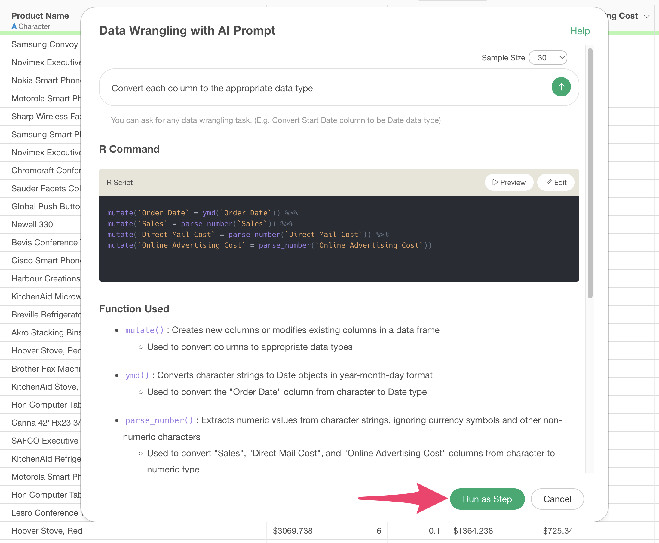
Code will be generated to convert each column to the appropriate data type. Check the explanation of the functions used and the expected results, then click the “Run as Step” button.
The step is added, and the “Order Date” column has been converted to Date type.
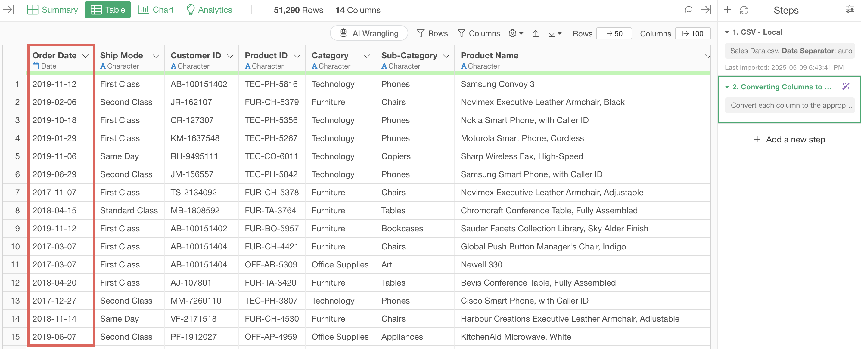
Also, the “Sales,” “Direct Mail Cost,” and “Online Ad Cost” columns have all been converted to Numeric type at once.
2. Creating Calculations
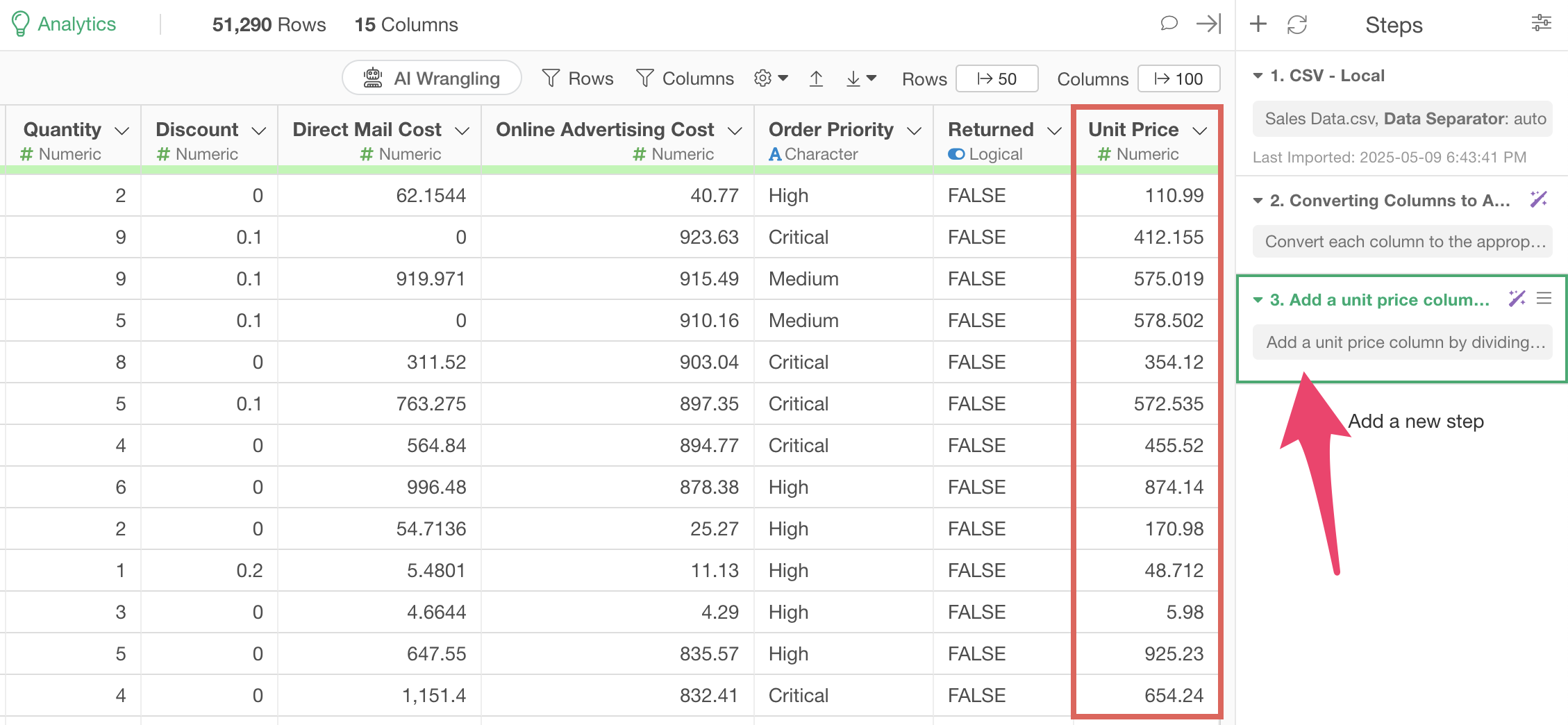
Next, we’ll create a new column “Unit Price” by dividing “Sales” by “Quantity”
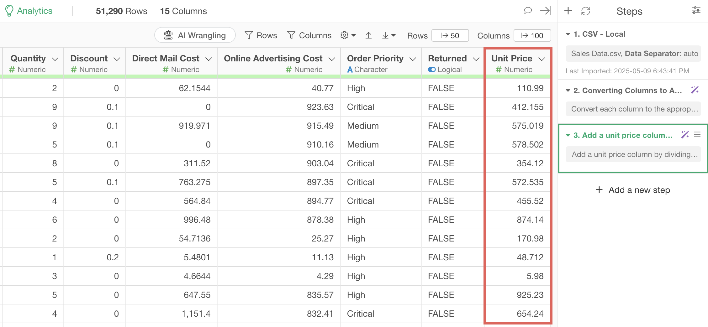
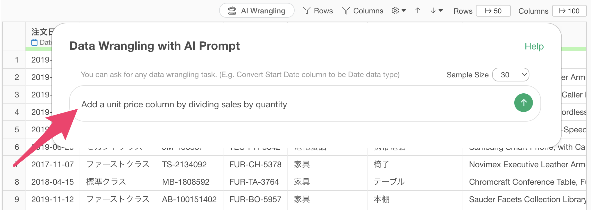
Click the “AI Wrangling” button, and when the AI Prompt dialog appears, enter the following text and execute:
Create a unit price column by dividing sales by quantity
Code will be generated to create a unit price column by dividing sales by quantity. Check the explanation of the functions used and the expected results, then click the “Run as Step” button.
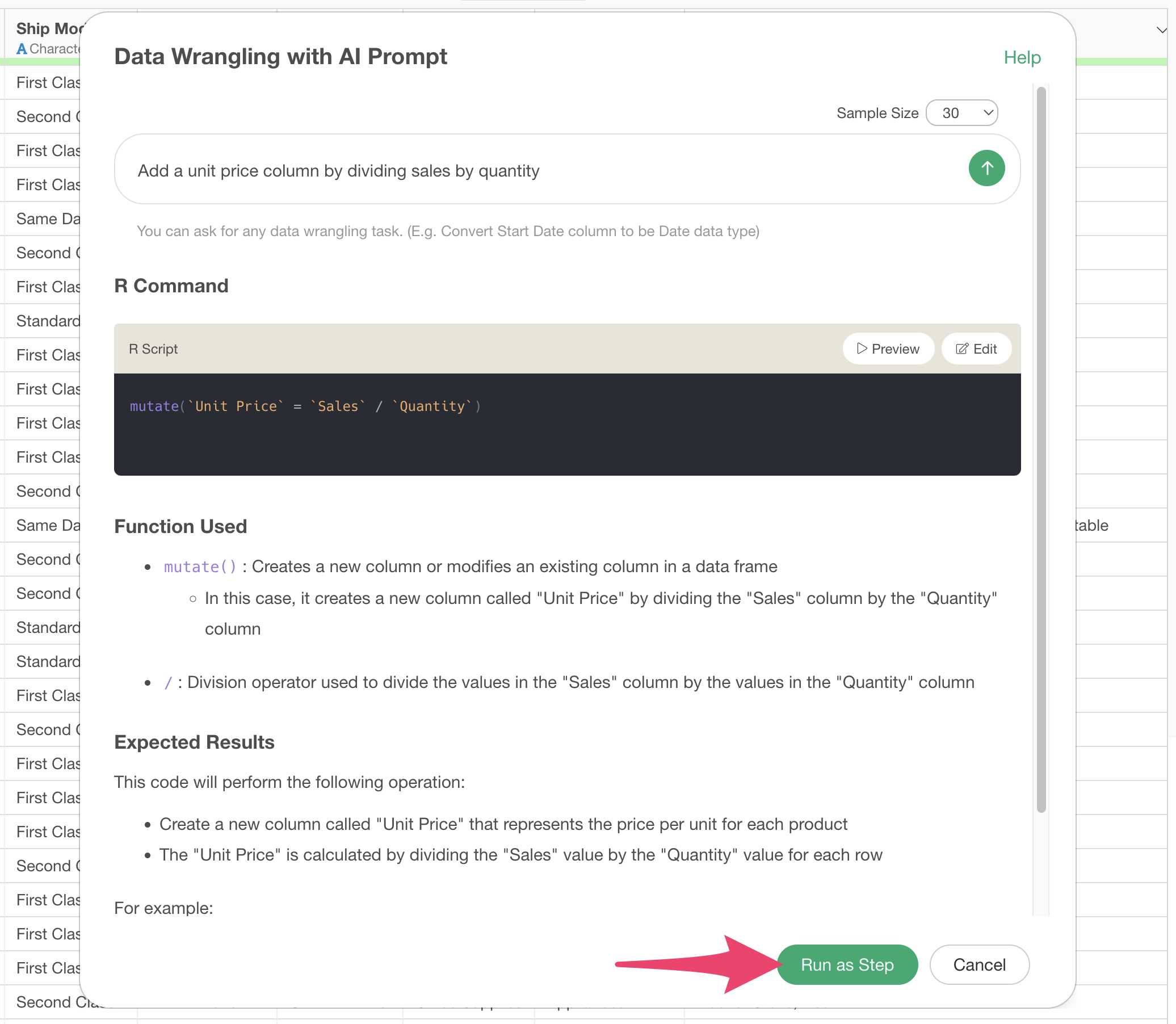
The step is added, and we’ve calculated the “Unit Price.”
3. Aggregating Data
The data we’re using has one row per product in each order, but we want to aggregate it to one row per customer with total sales and number of orders.
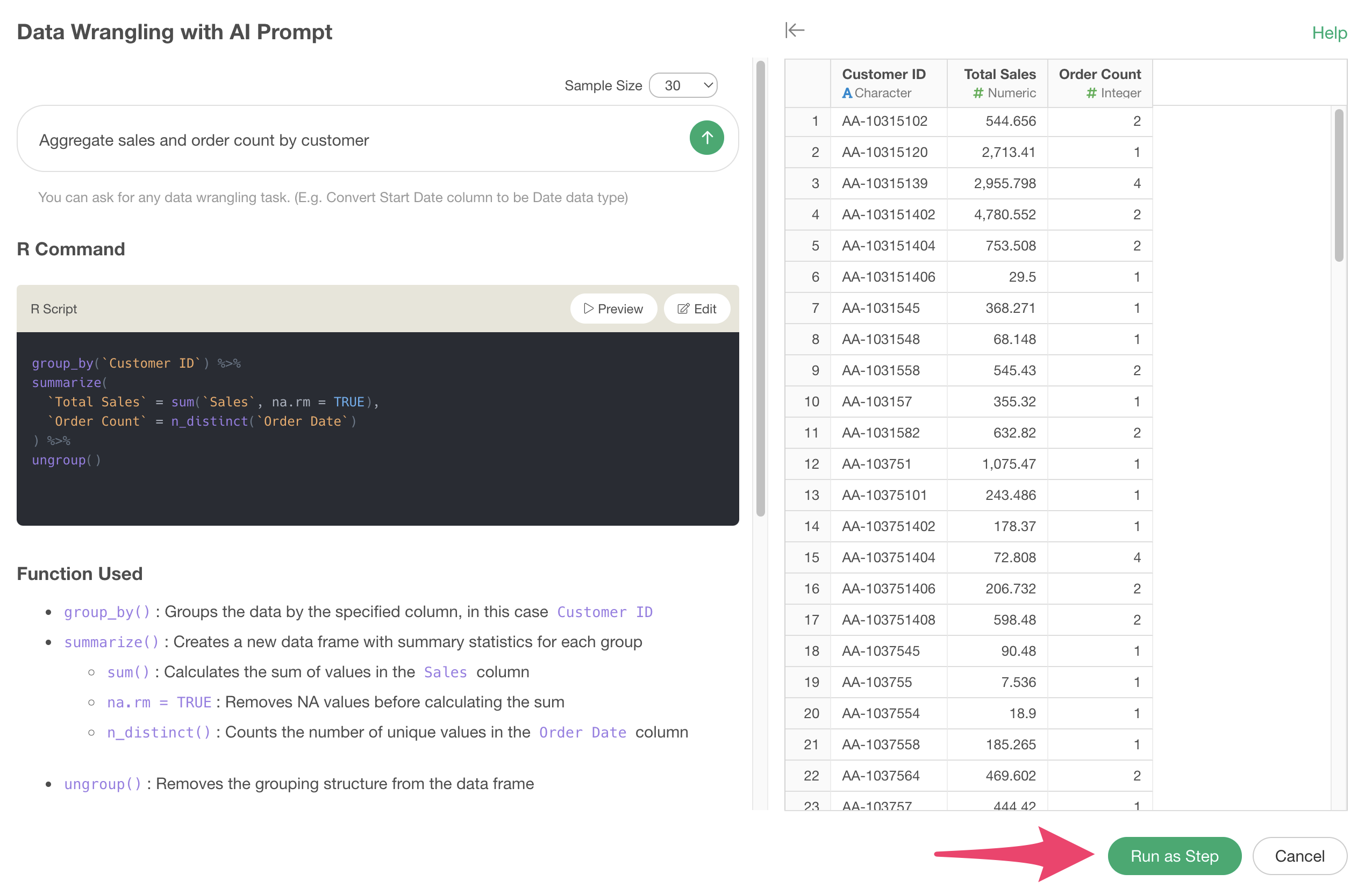
Click the “AI Wrangling” button, and when the AI Prompt dialog appears, enter the following text and execute:
Aggregate sales and order count by customer
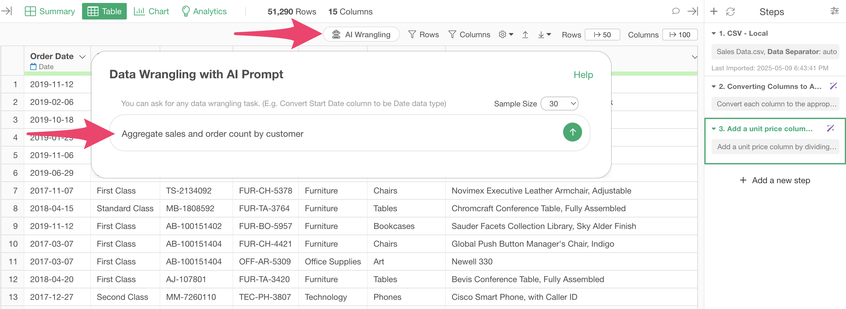
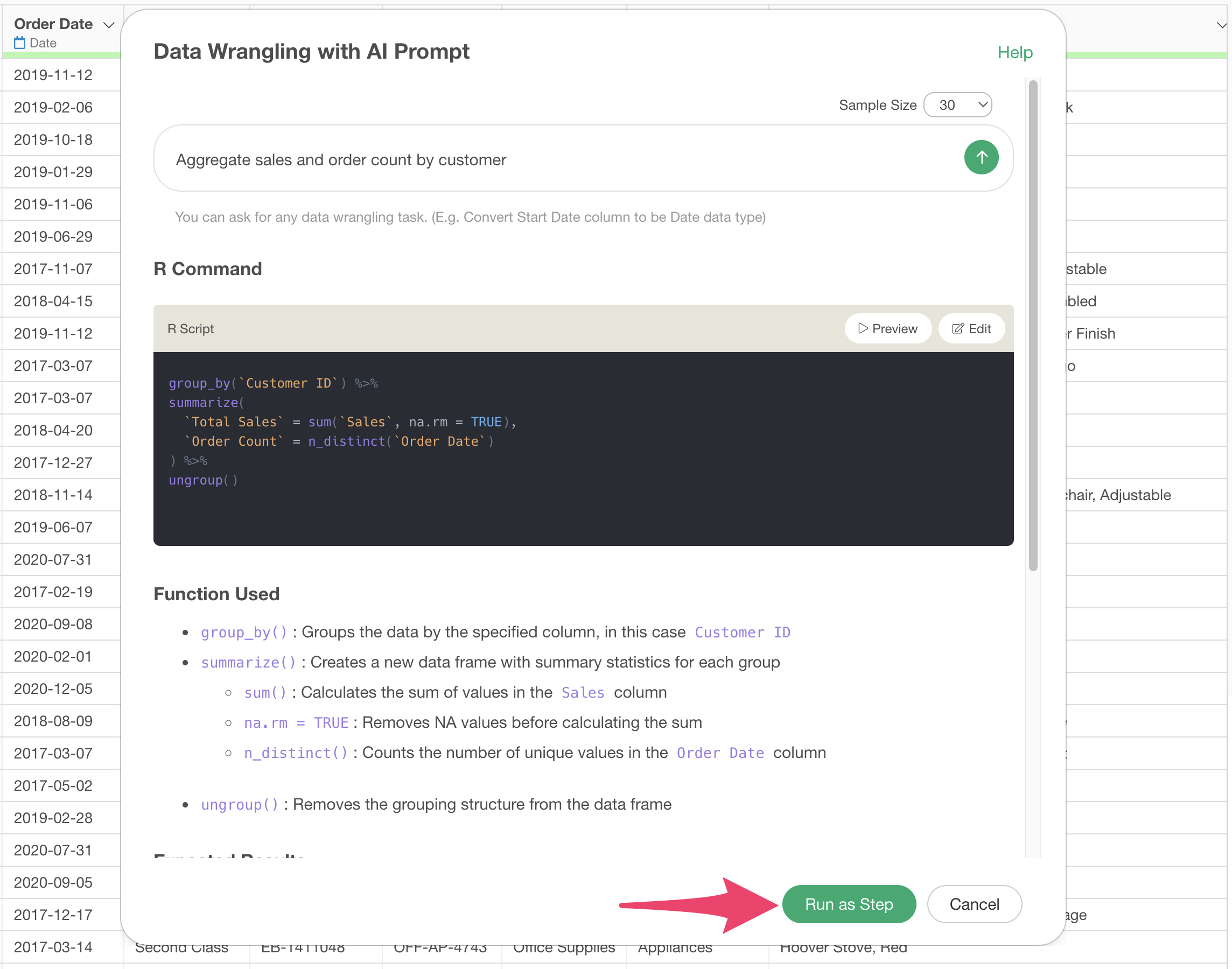
Code will be generated to aggregate total sales and order count by customer ID.
At this point, you can click the Preview button to check the results of the prompt execution.
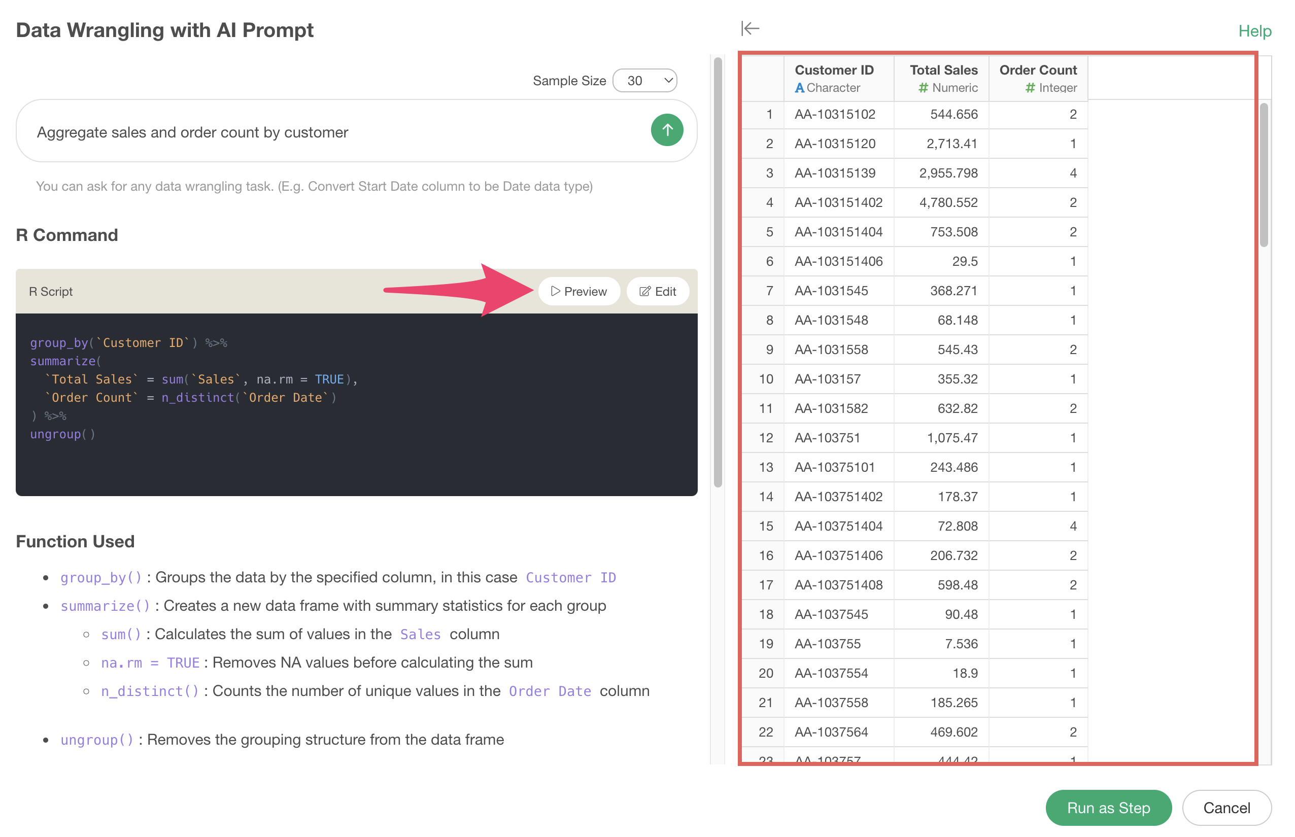
After confirming the results, click the “Run as Step” button.
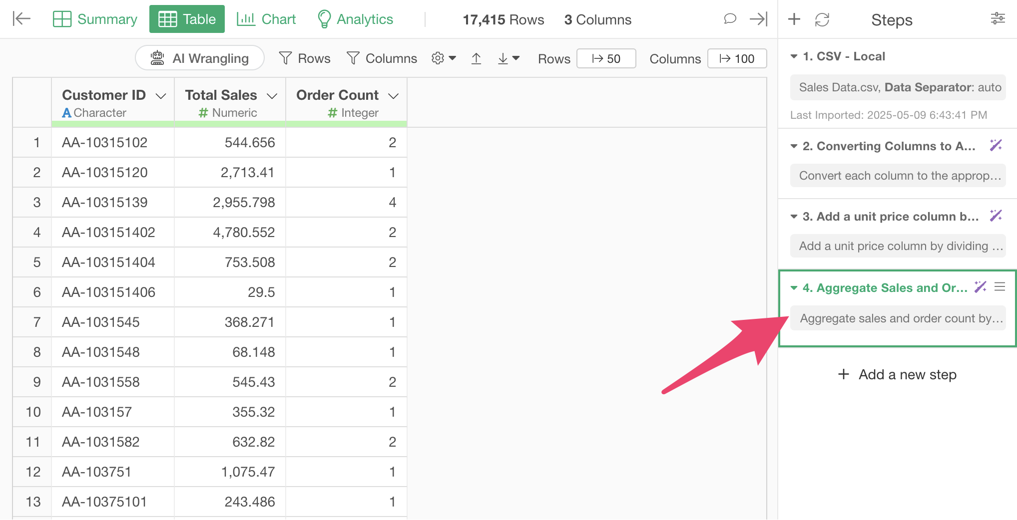
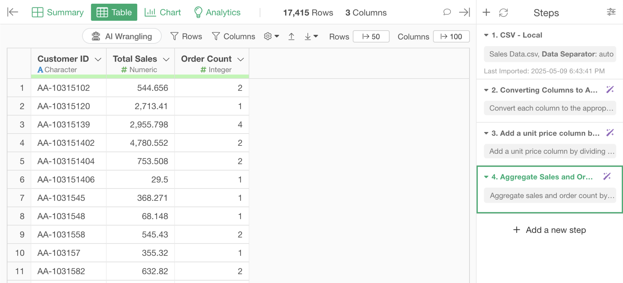
The step is added, and the data has been aggregated from one row per line item to one row per customer, showing total sales and order count per customer.
4. Joining Data
Let’s import customer attribute data separately from the sales data we’ve been using.
The customer attribute data has one row per customer, with columns for customer attribute information such as the region where the customer lives and their segment.
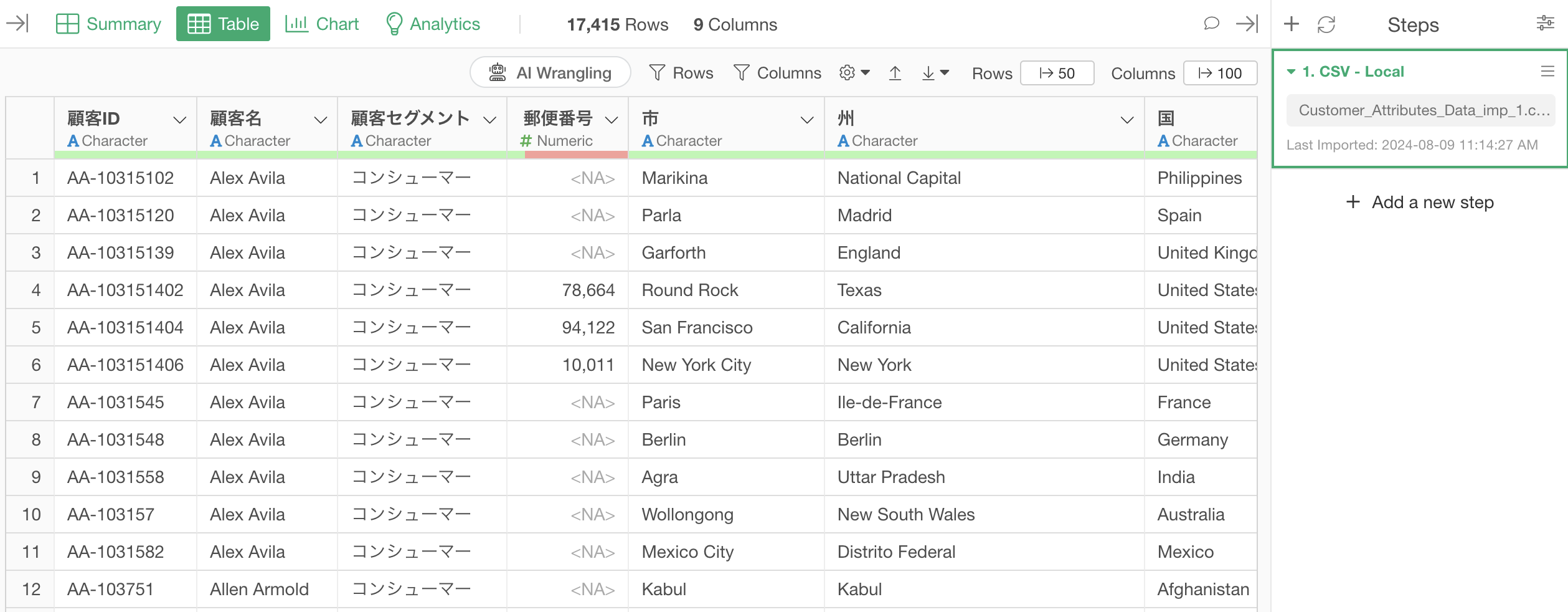
You can download the data from this page, and import it the same way as the sales data.
Now we want to add the customer attribute data as columns to the data we aggregated earlier.
 This
kind of joining process can also be handled with “AI Prompt.”
This
kind of joining process can also be handled with “AI Prompt.”
Click the “AI Wrangling” button and type “$” in the prompt dialog to display a list of dataframes in the project.
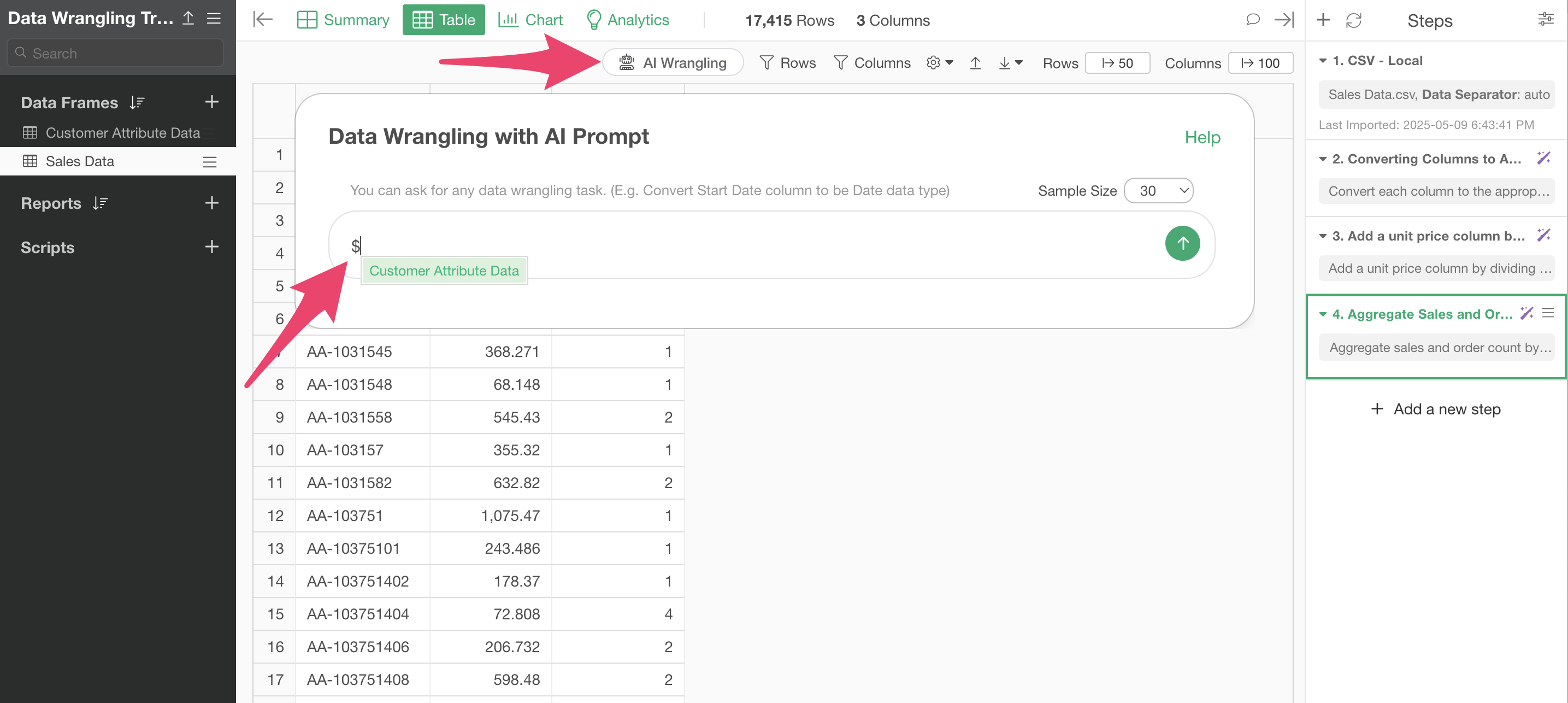
When you want to perform operations that reference other dataframes, such as joining, enter “$” like this to specify a dataframe in the project.
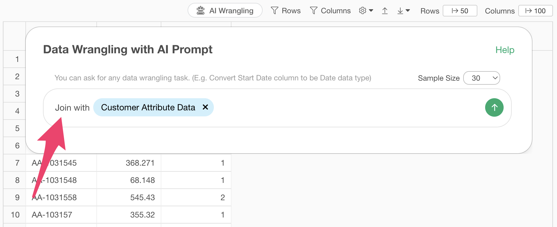
Since we want to join the customer attribute data, enter the following text and execute:
Join with Customer Attribute Data
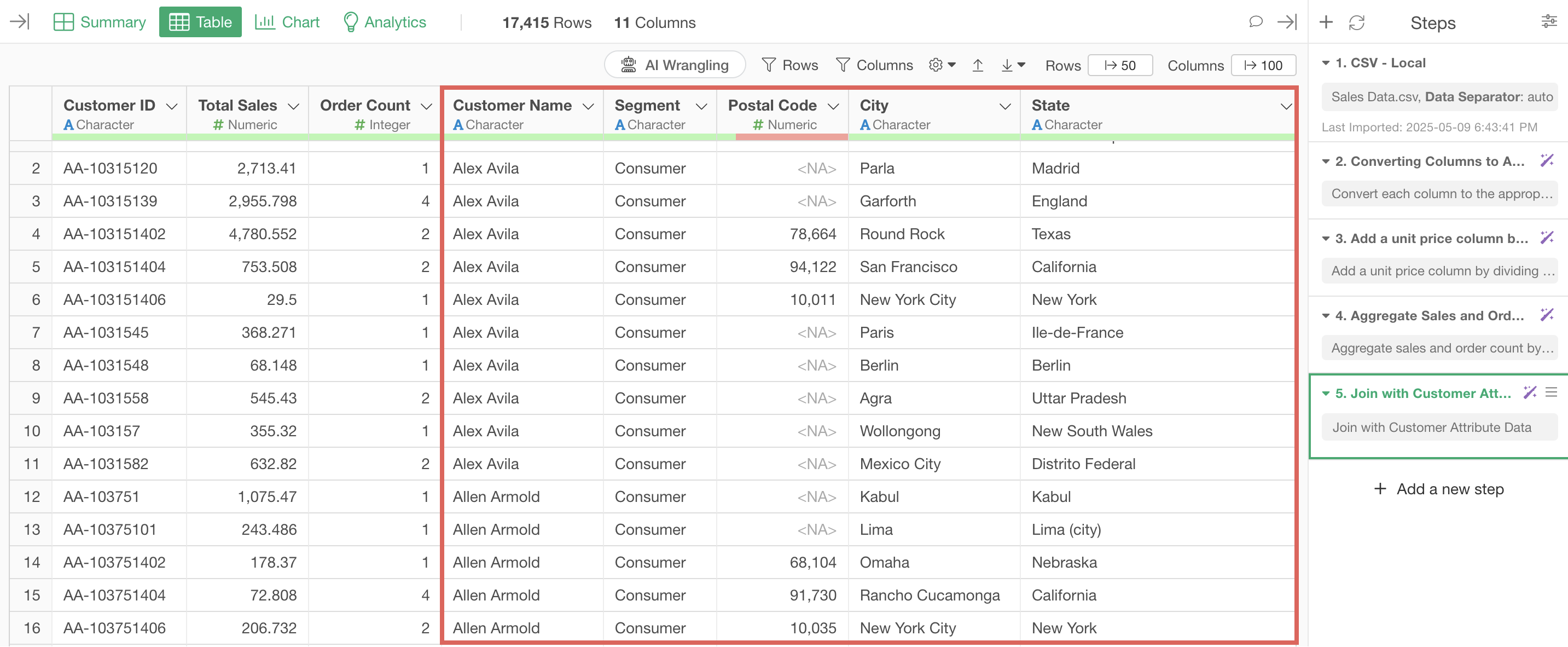
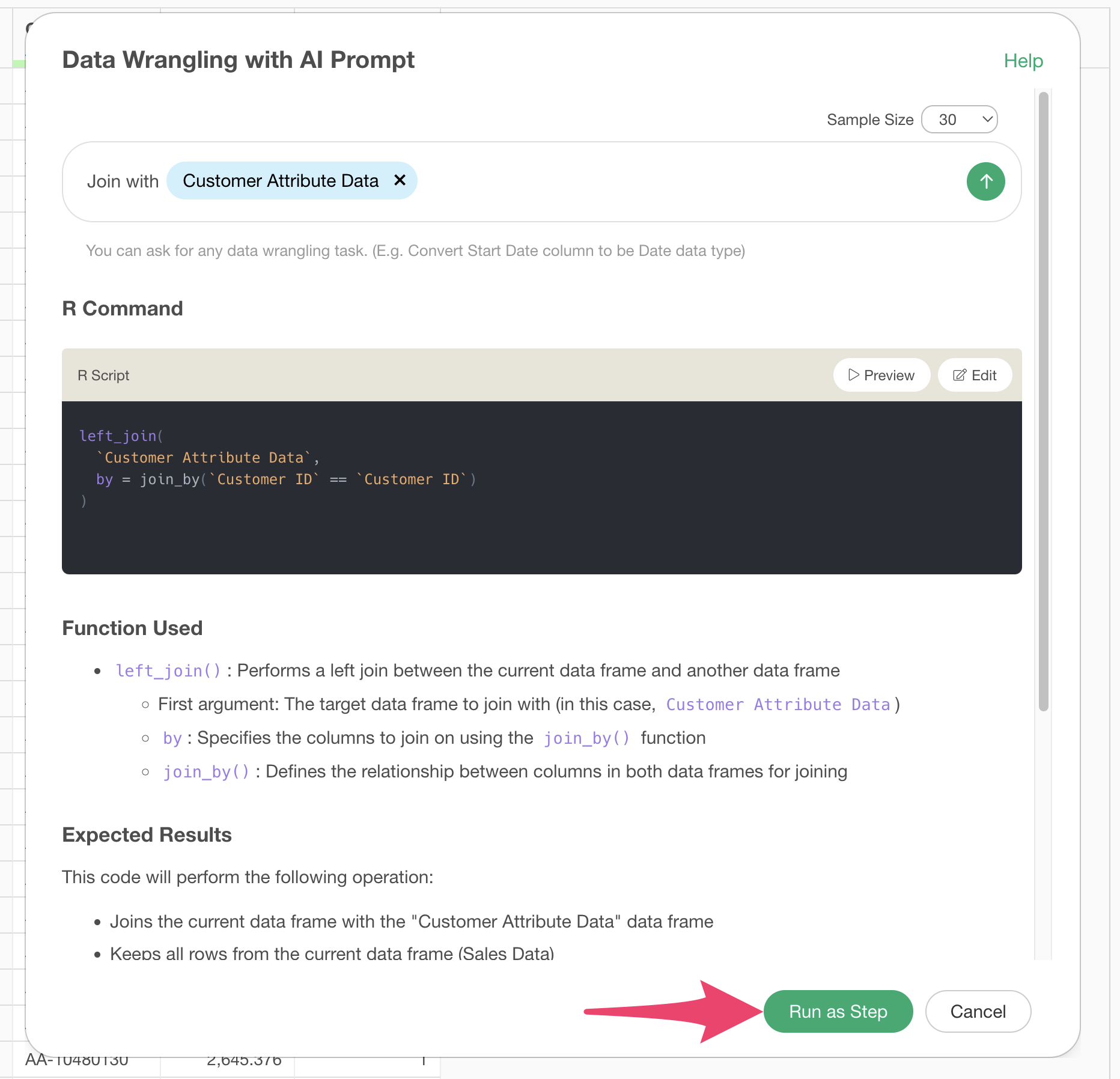
Code will be generated to join the customer attribute data with the current data. Check the explanation of the functions used and the expected results, then click the “Run as Step” button.
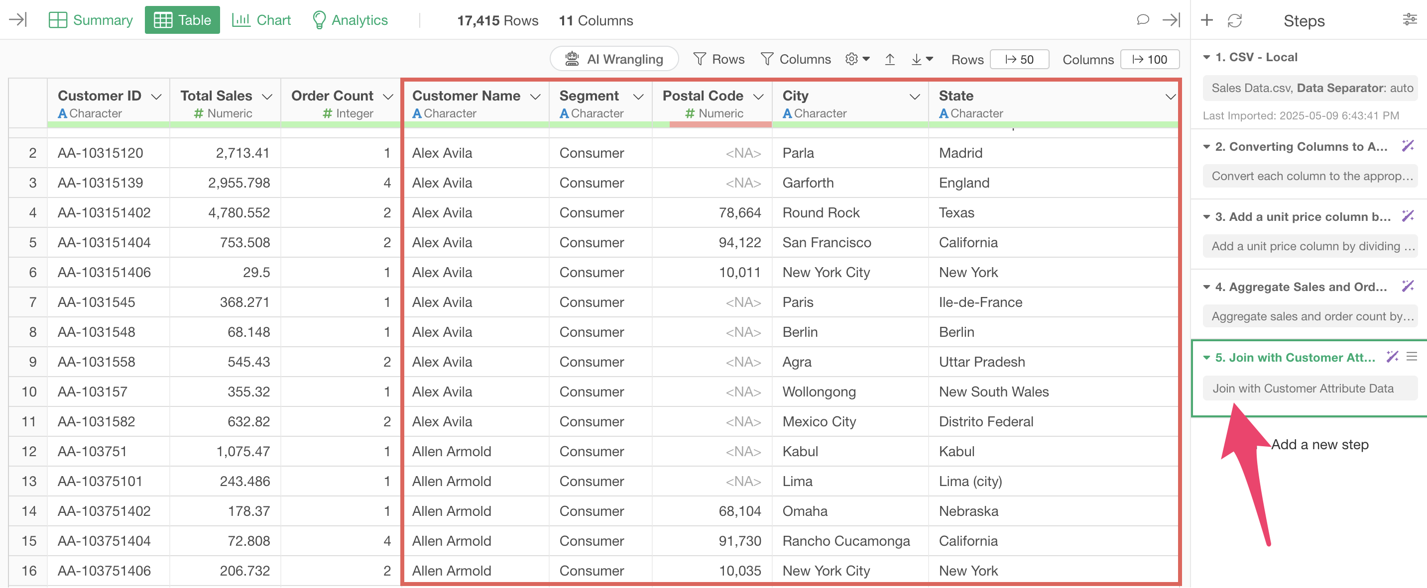
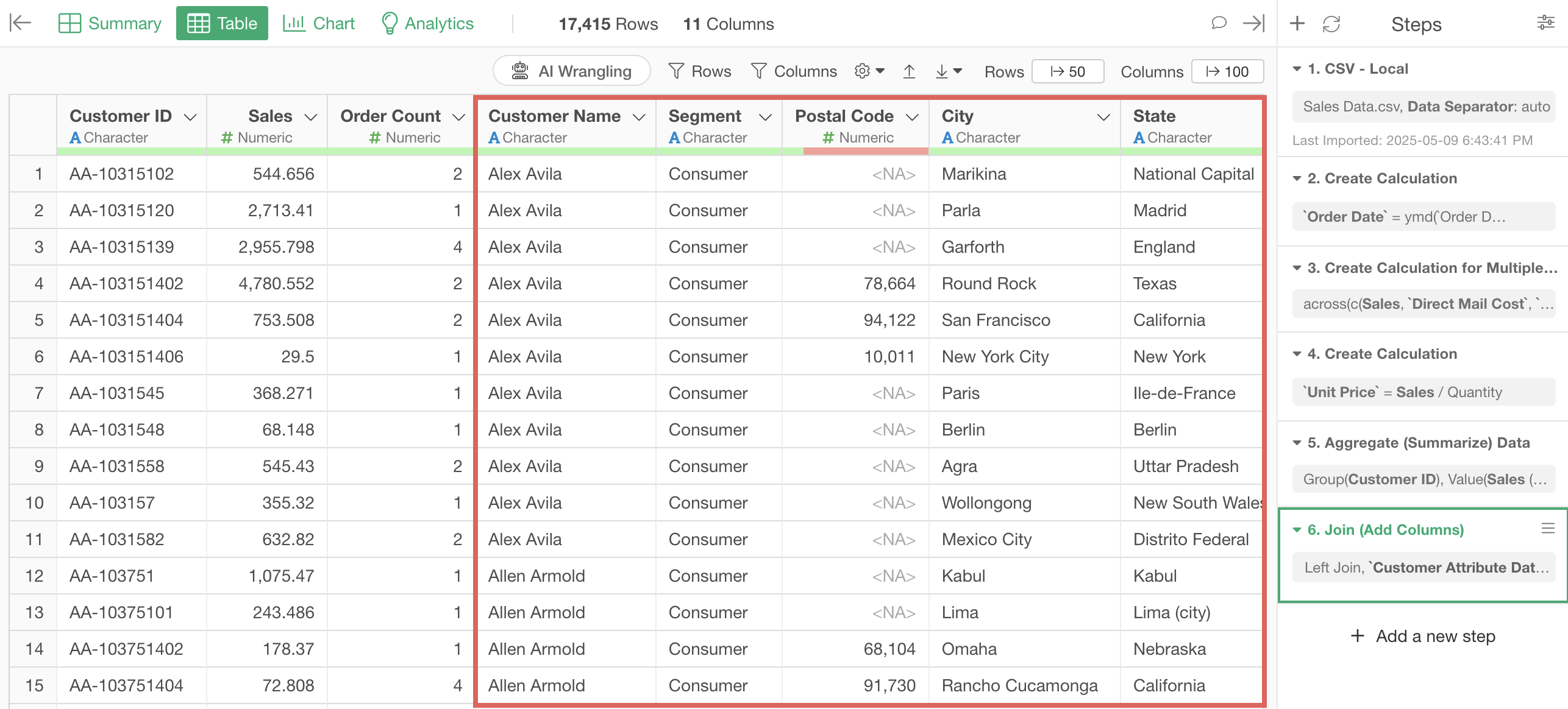
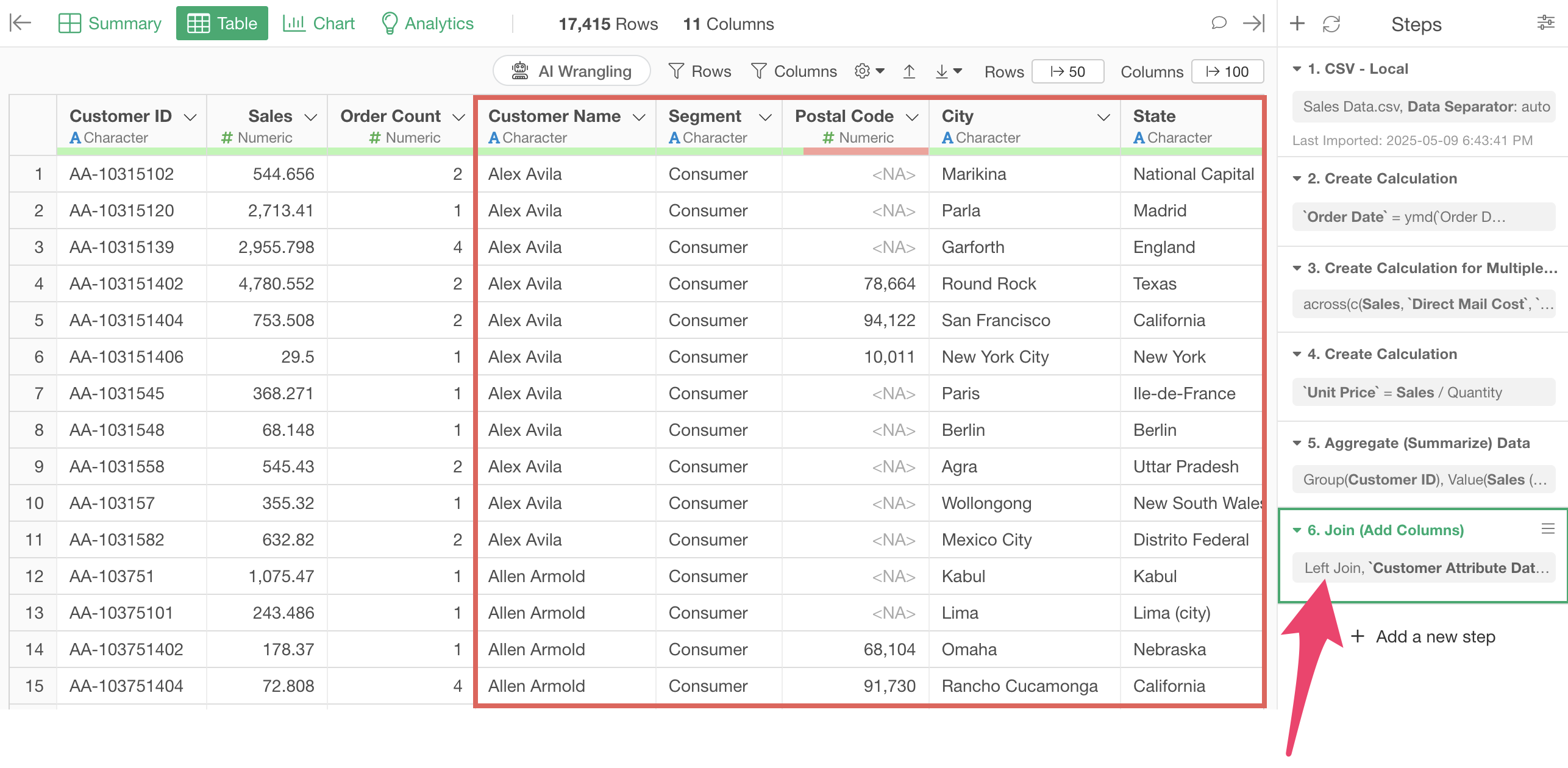
The step is added, and customer attribute information columns (region, segment, etc.) have been added to the customer sales data.
Processing Data with UI
1. Converting Data Types
The order date column is currently a string type, but we want to convert this data to a date type.

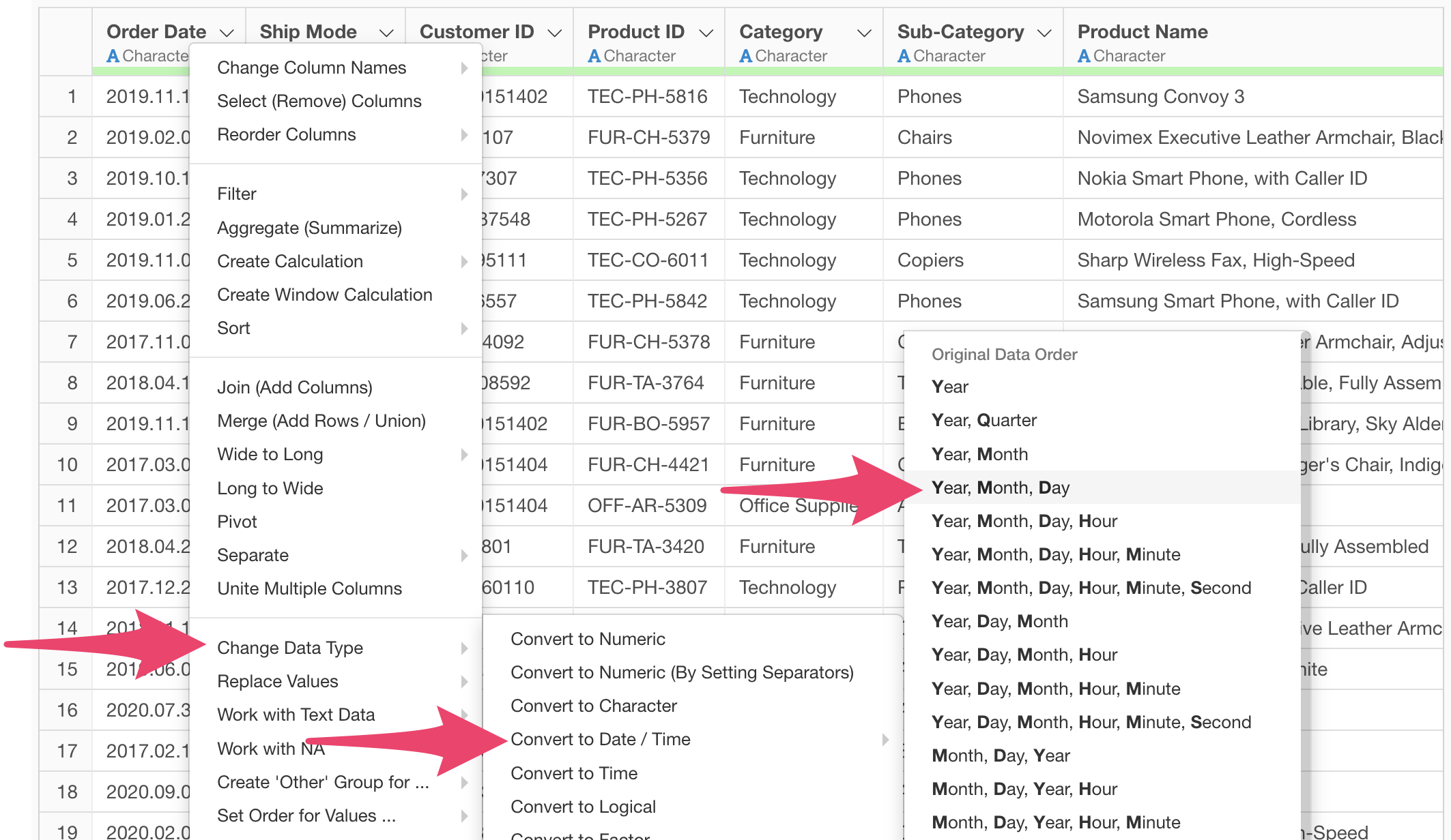
From the order date column, select “Convert Data Type” > “Convert to Date/Time”. Then, based on the date order, select “Year, Month, Day.”
The calculation editor already has the ymd function for converting to date type, so just click the execute button.
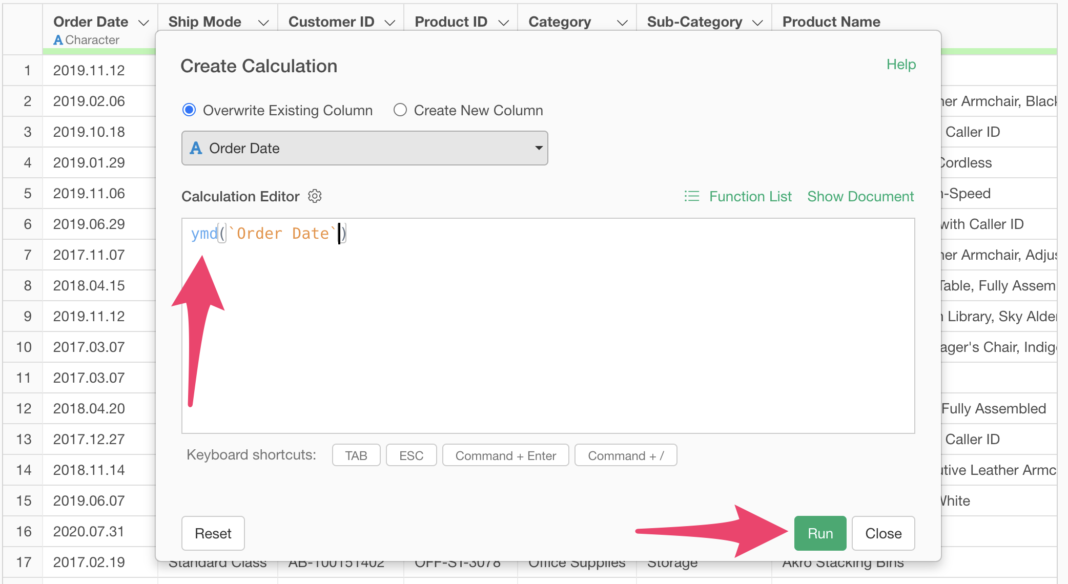
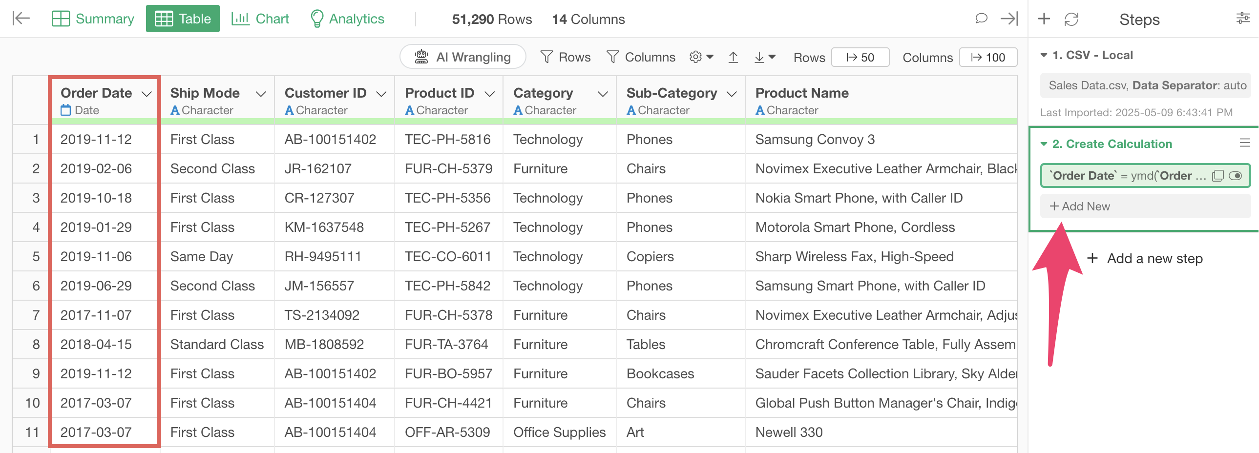
We’ve successfully converted the order date column to Date type.
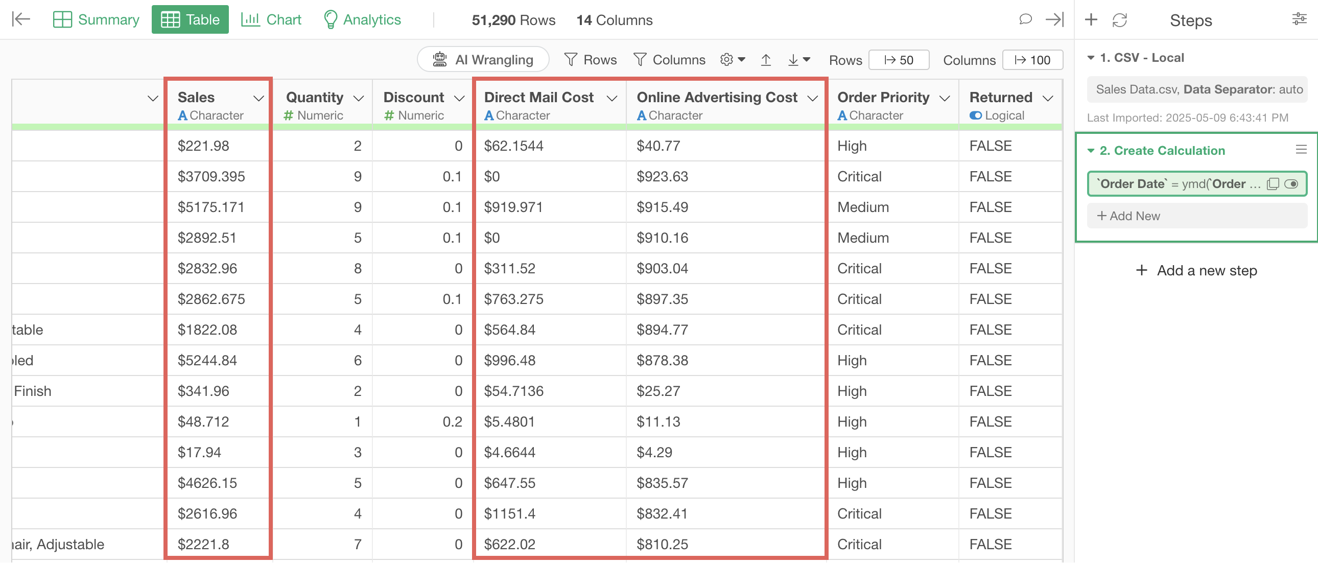
There are other columns that should have their data types changed as well.
These are the “Sales,” “Direct Mail Cost,” and “Online Advertising Cost” columns. These should properly be Numeric type, but because they contain characters ($) within the numbers, they are Character type.
Let’s convert all these columns to Numeric type at once.
Hold down the Command key on Mac or Ctrl key on Windows while selecting the three columns “Sales,” “Direct Mail Cost,” and “Online Ad Cost,” then select “Convert Data Type” > “Convert to Numeric Type” from the column header menu.
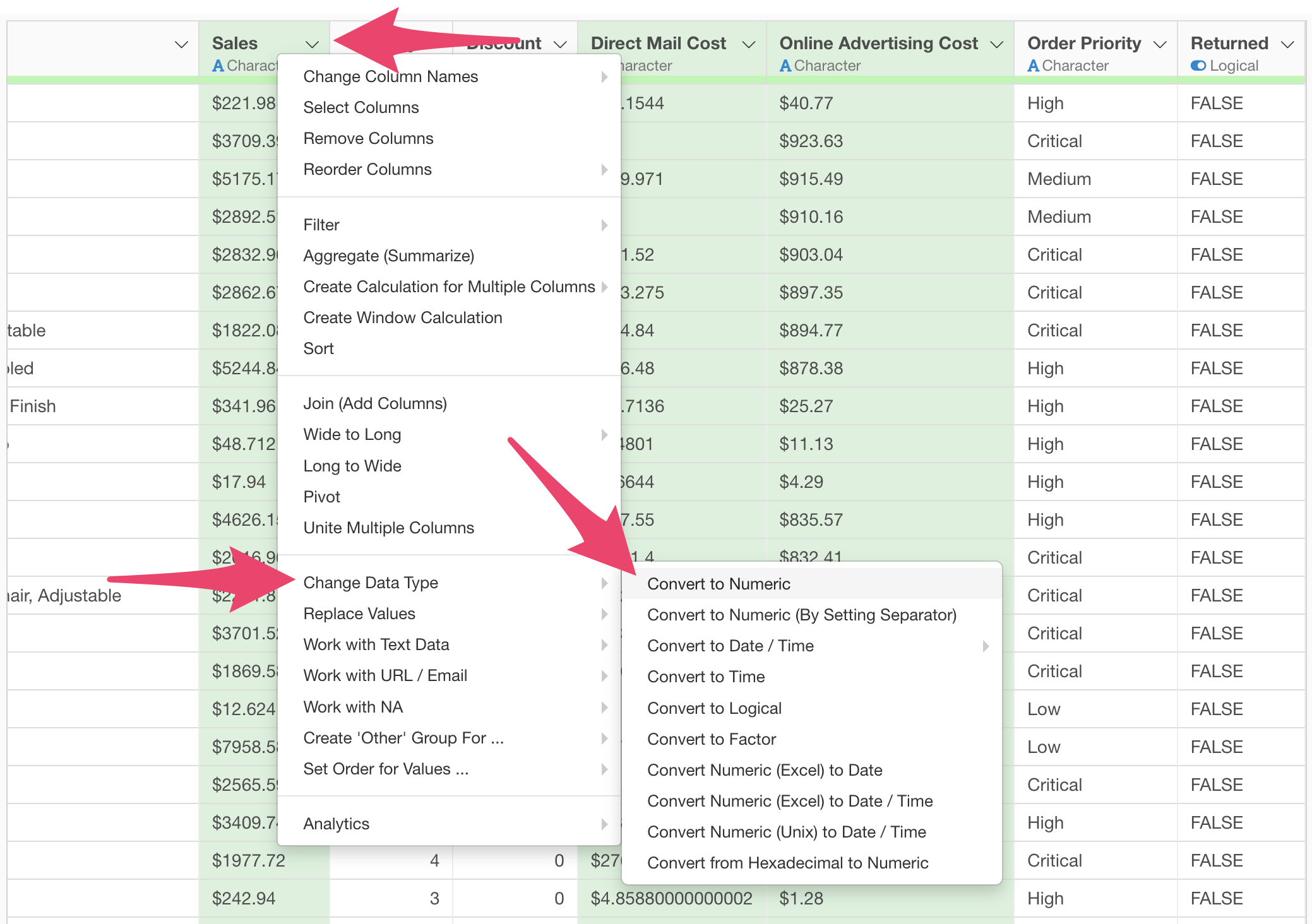
A dialog for creating calculations for multiple columns will appear, so click the “Execute” button.
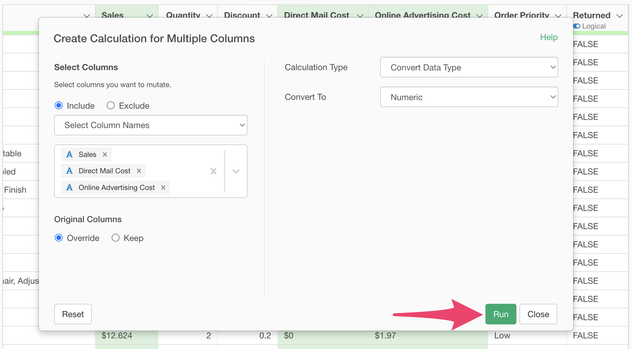
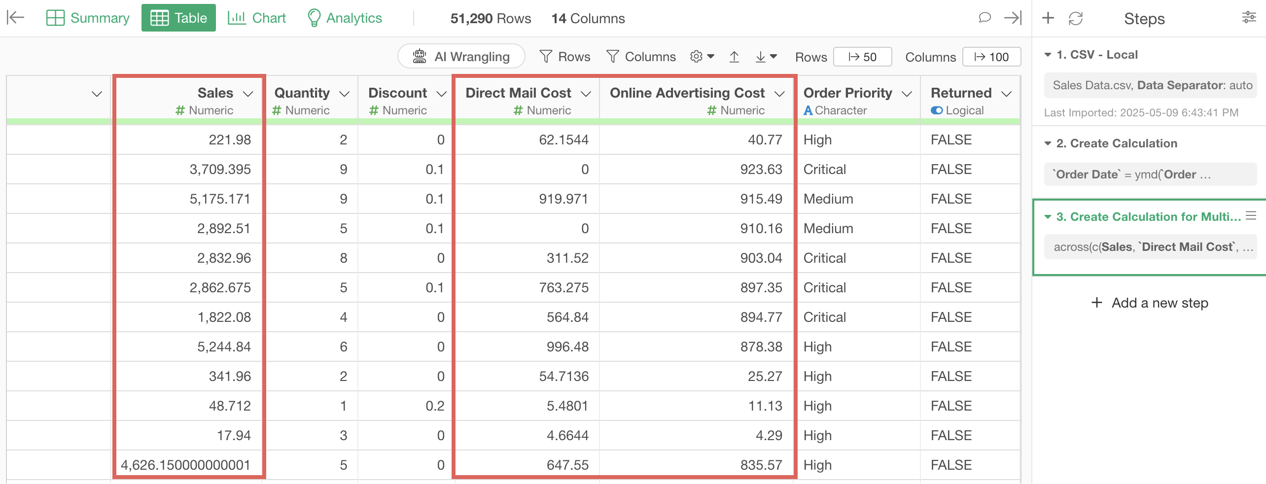
By executing, you can see that the three columns “Sales,” “Direct Mail Cost,” and “Online Ad Cost” have been converted to Numeric type.
2. Creating Calculations
Let’s say we want to create a new column “Unit Price” by dividing “Sales” by “Quantity.”
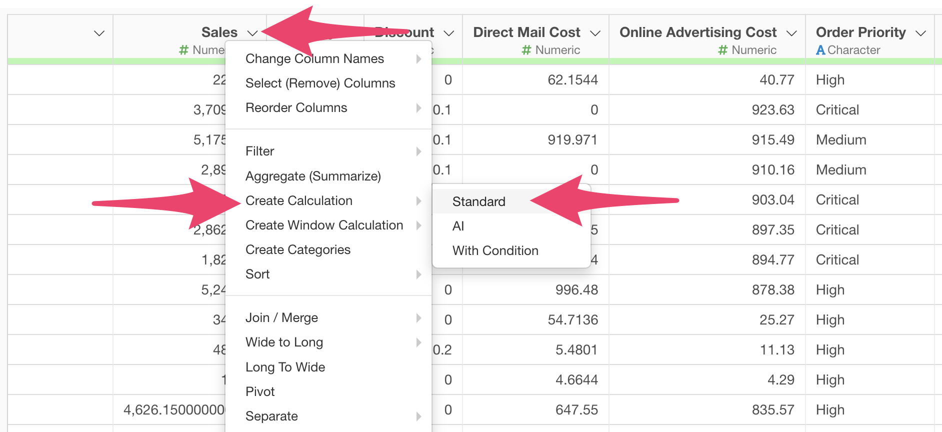
For this, select “Create Calculation” > “Standard” from the column header menu.
When the Create Calculation dialog appears, enter the following expression in the calculation editor:
Sales / Quantity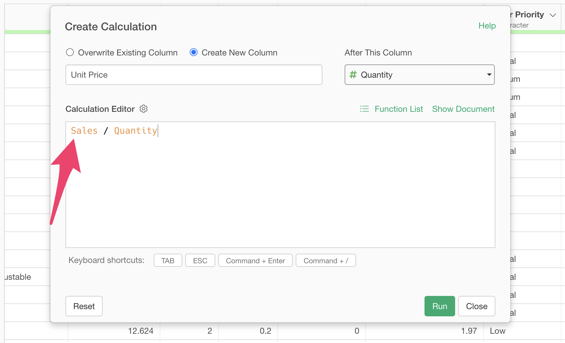
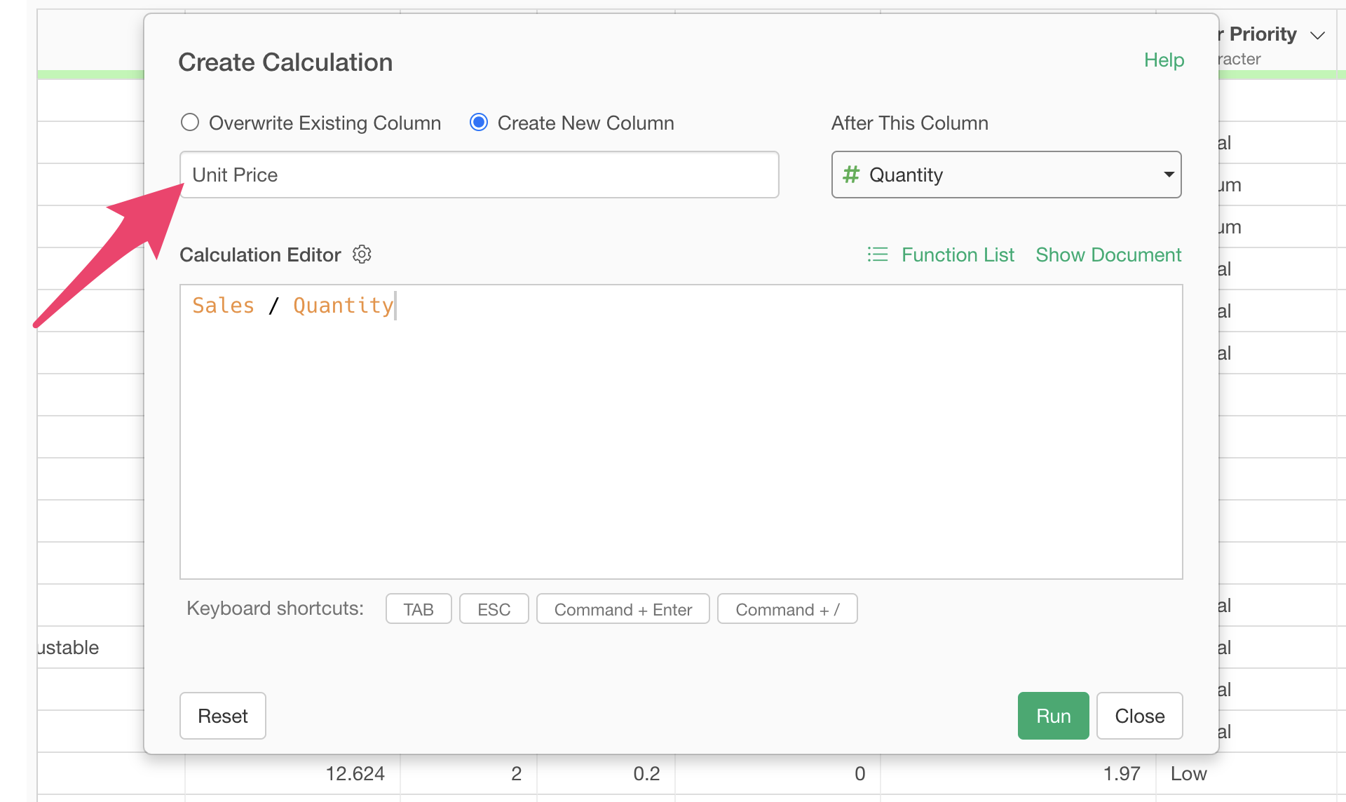
Check “Create new column” and specify “Unit Price” as the column name.
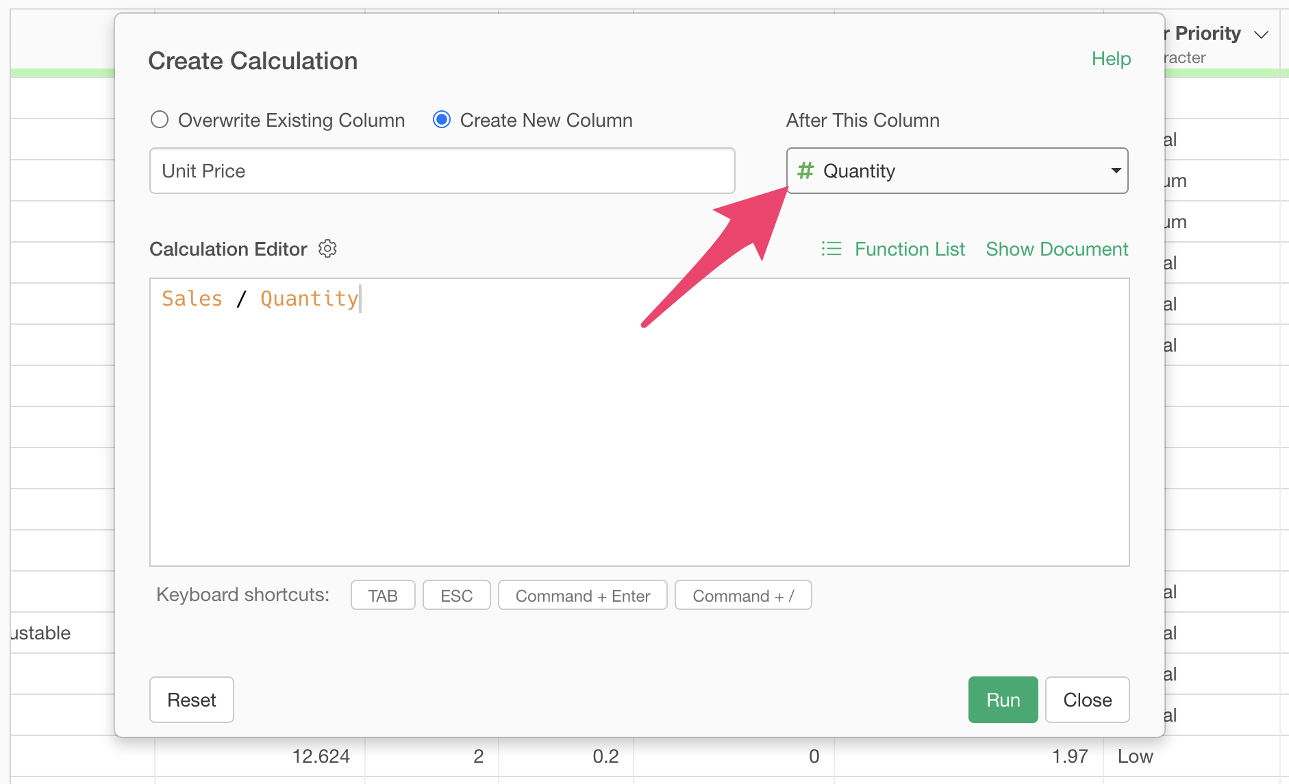
In “Create after this column,” you can specify the position of the newly created column. In this case, we want to create the “Unit Price” column after “Quantity,” so select “Quantity.”
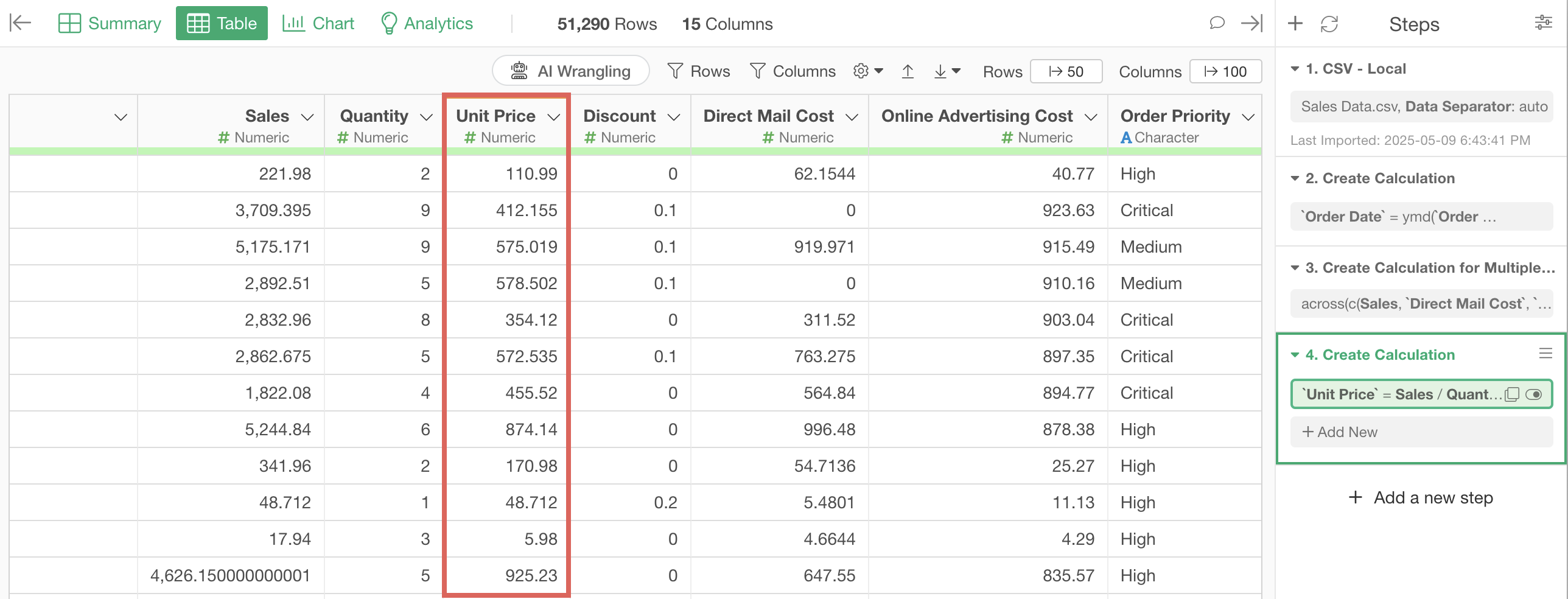
By executing, we’ve successfully created the “Unit Price” column.

3. Aggregating Data
The data we’re using has one row per product in each order, but we want to aggregate it to one row per customer to calculate total sales and order count.
To aggregate data, select “Aggregate” from the Customer ID column header menu.
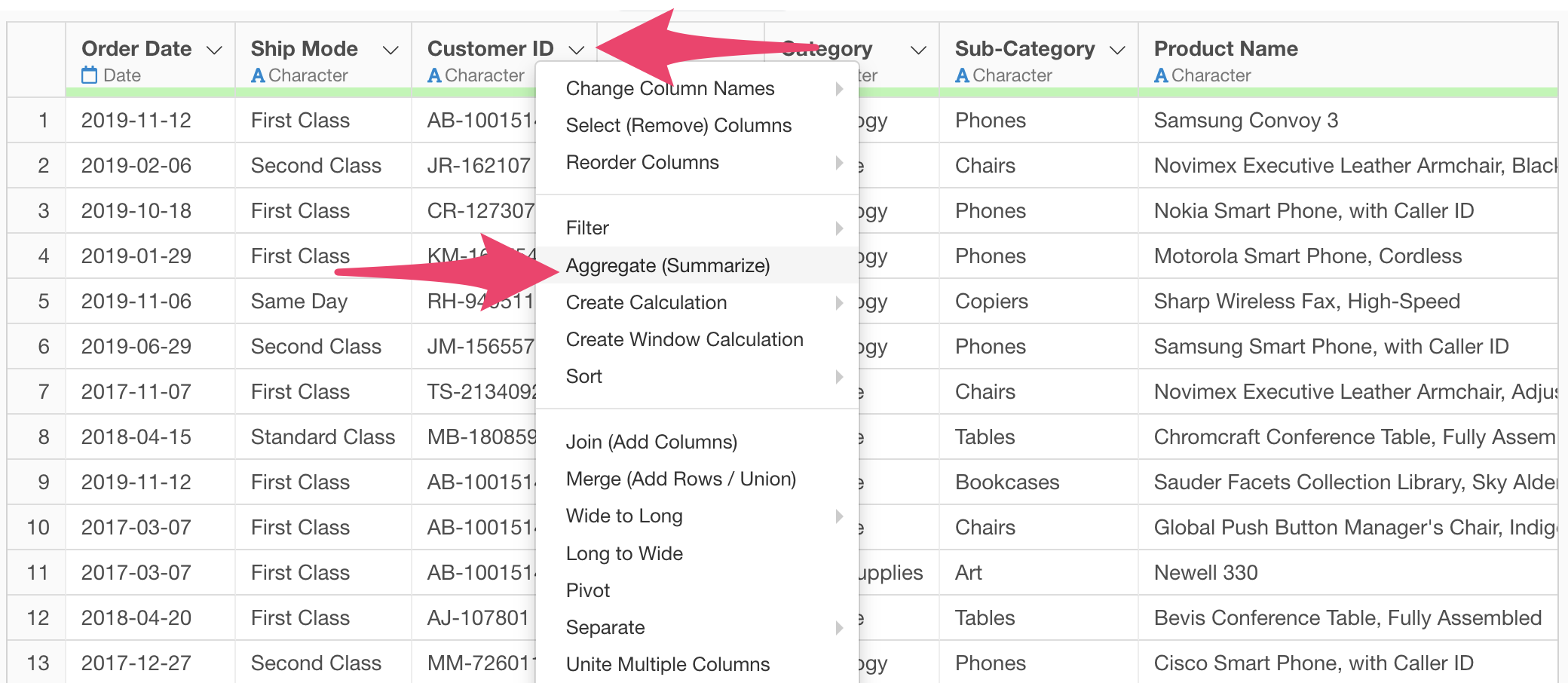
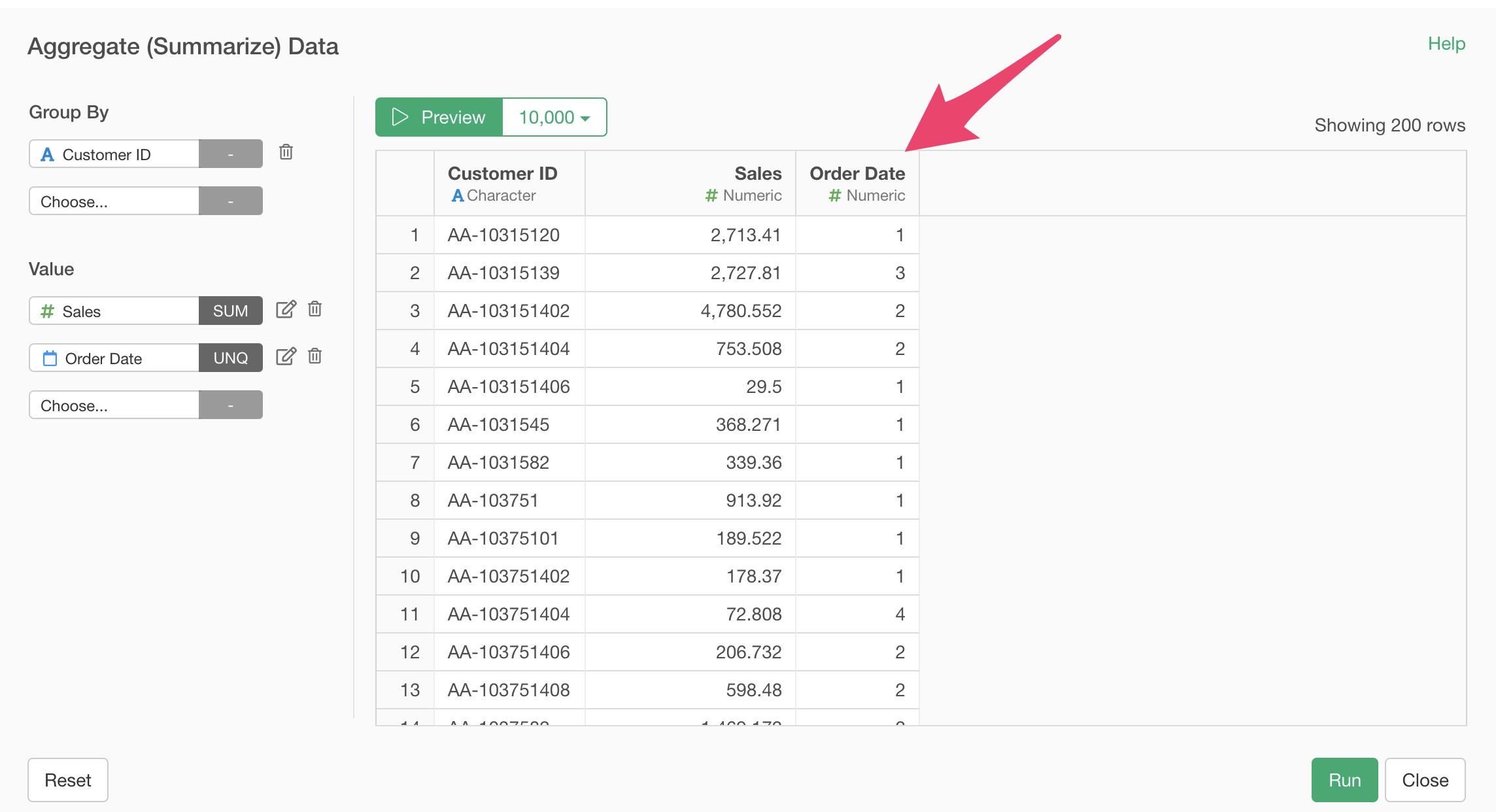
The Aggregate dialog appears with the “Customer ID” column assigned to the group.
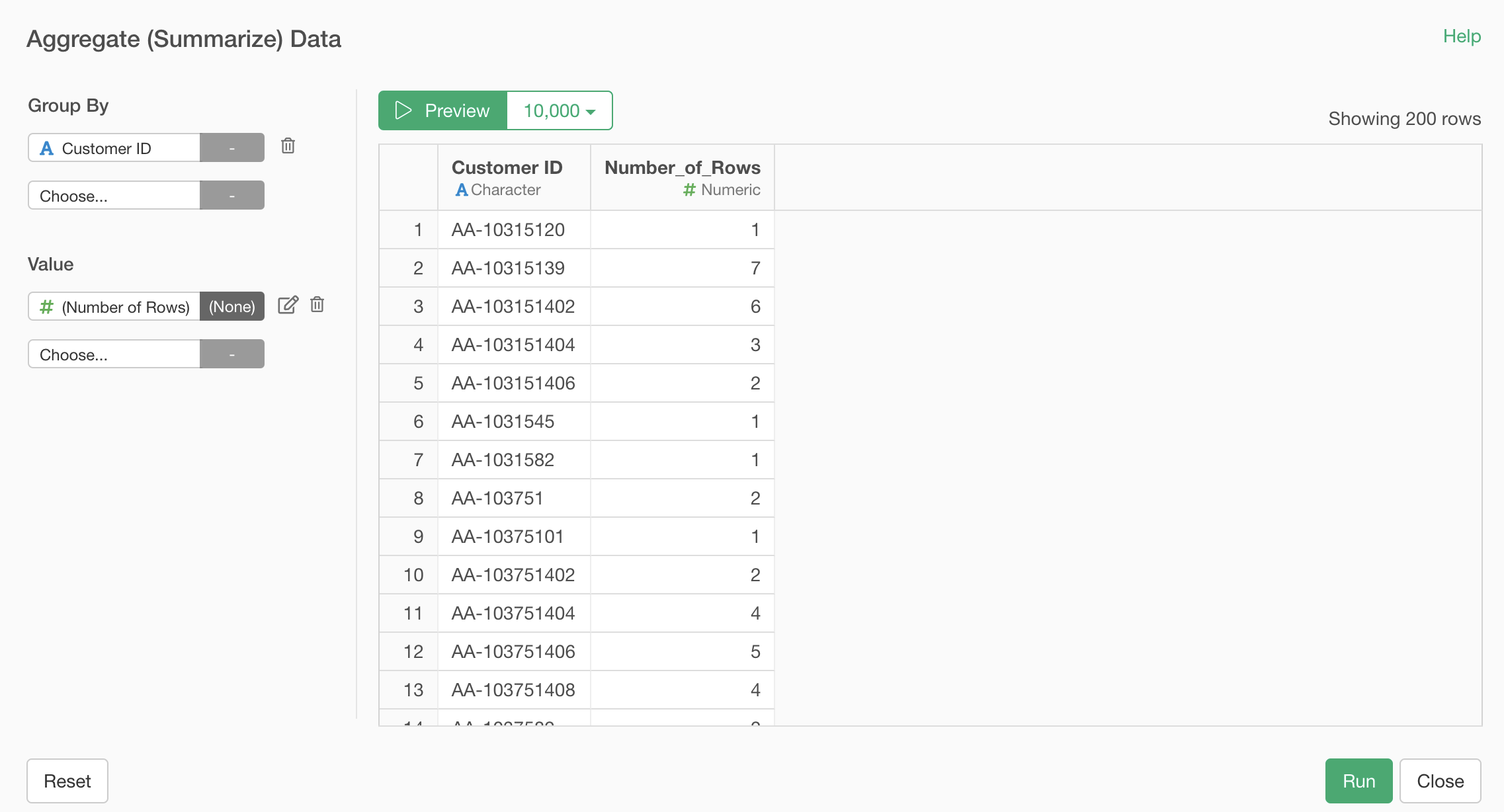
Assign the “Sales” column to the value and select “SUM” as the aggregation function.
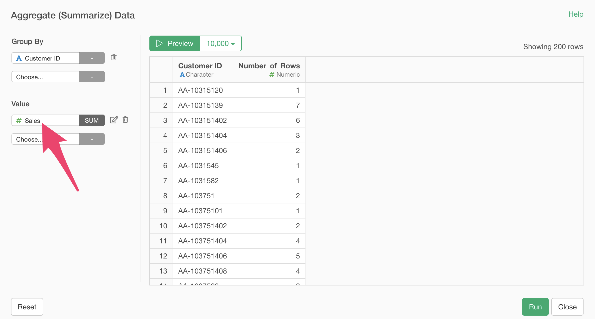
Next, for the second value, we want to calculate the order count.
To calculate the order count, select “Order Date” for the value and “Unique Count” for the aggregation function.
This allows us to count orders even if there are multiple rows for the same customer on the same order date, counting them as the same order.
However, the column name is still “Order Date,” so let’s change it.
Click the “Edit” button next to “Order Date” in the value section, and specify “Order Count” as the new column name.
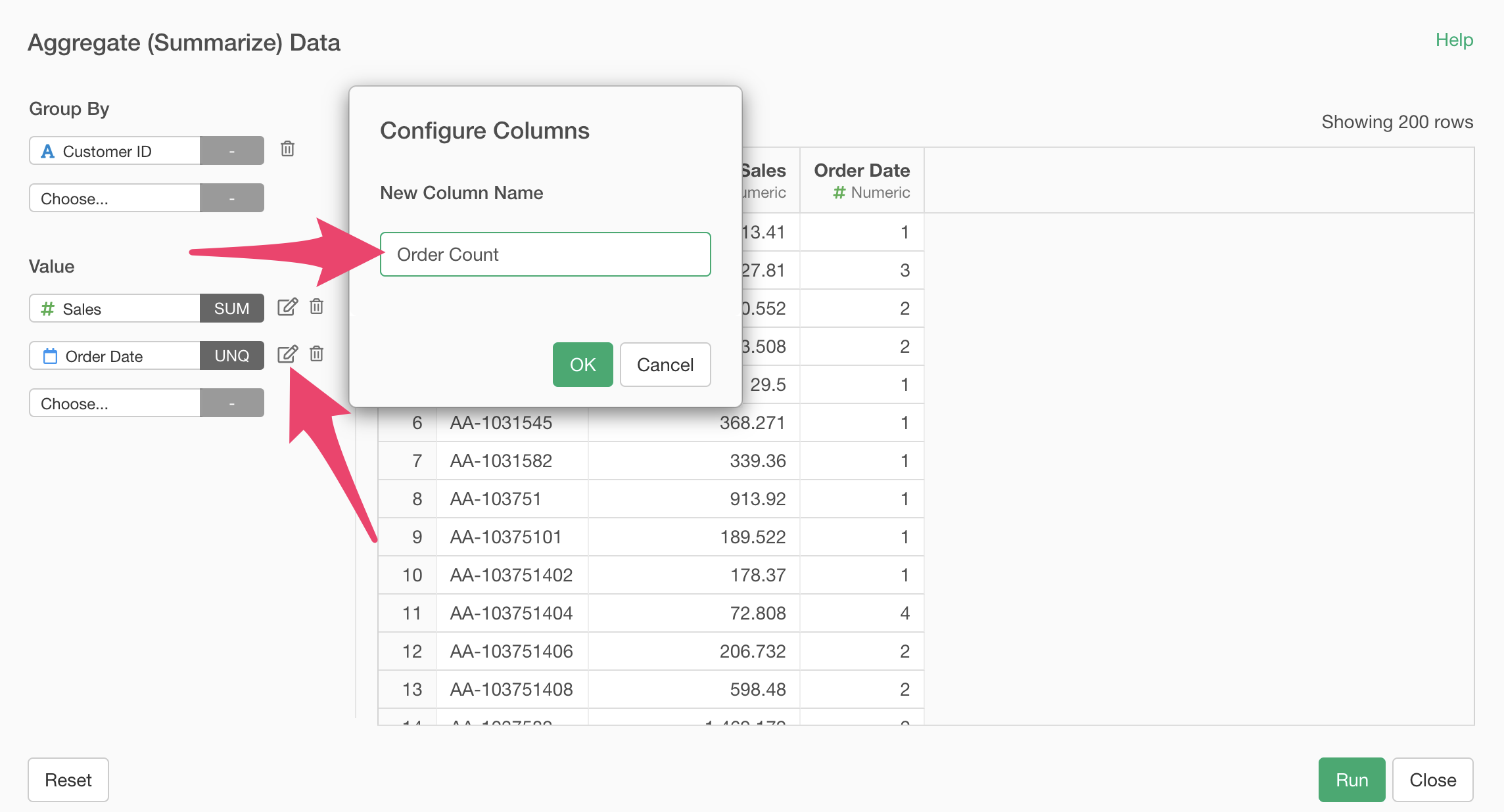
Now that we’ve changed the column name to “Order Count,” click the “Execute” button.
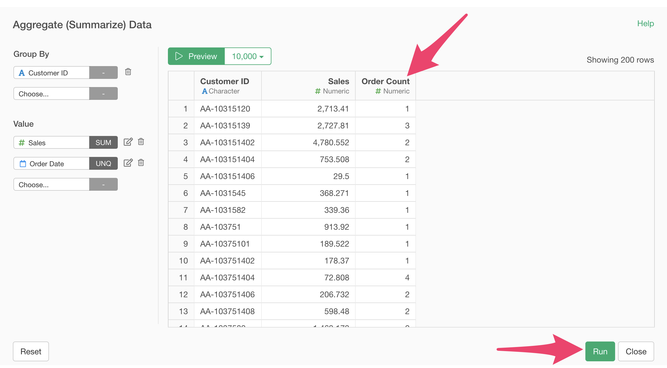
We’ve successfully aggregated from one row per line item to one row per customer.
4. Joining Data
Let’s import customer attribute data separately from the sales data we’ve been using.
The customer attribute data has one row per customer, with columns for customer attribute information such as the region where the customer lives and their segment.

You can download the data from this page, and import it the same way as the sales data.
Now we want to add the customer attribute data as columns to the data we aggregated earlier.
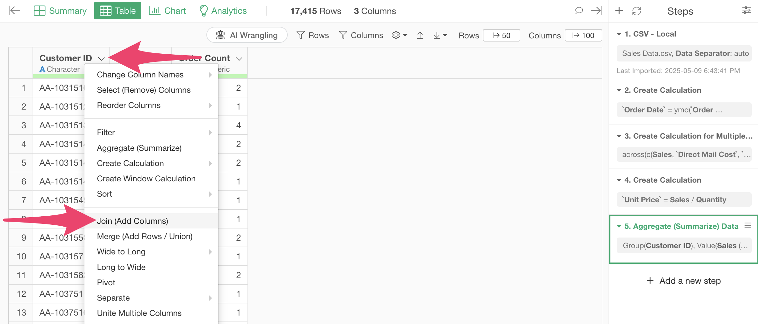
We want to add the customer attribute data we just imported as columns to this sales data.
Select “Join” from the Customer ID column of the sales data.
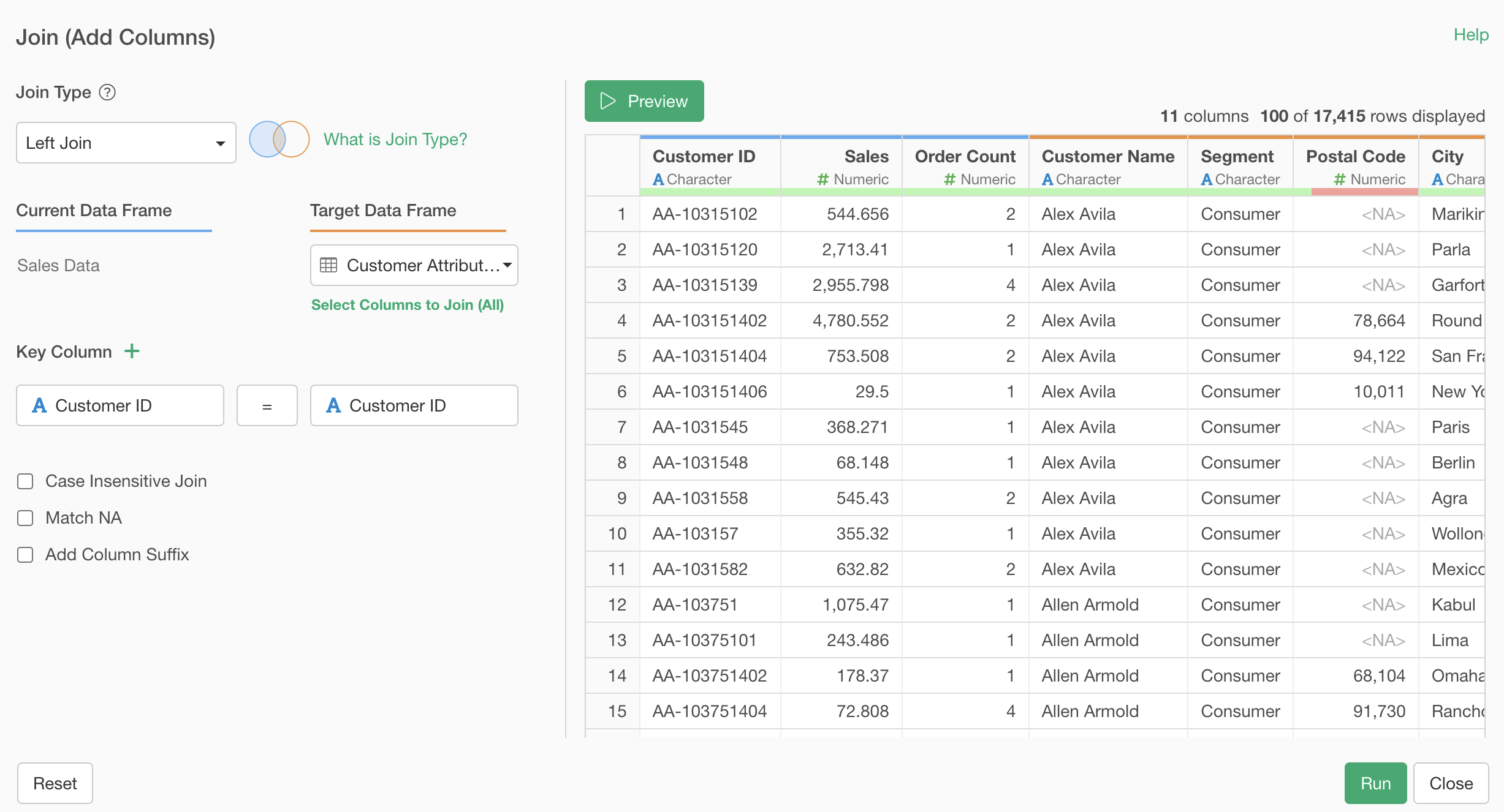
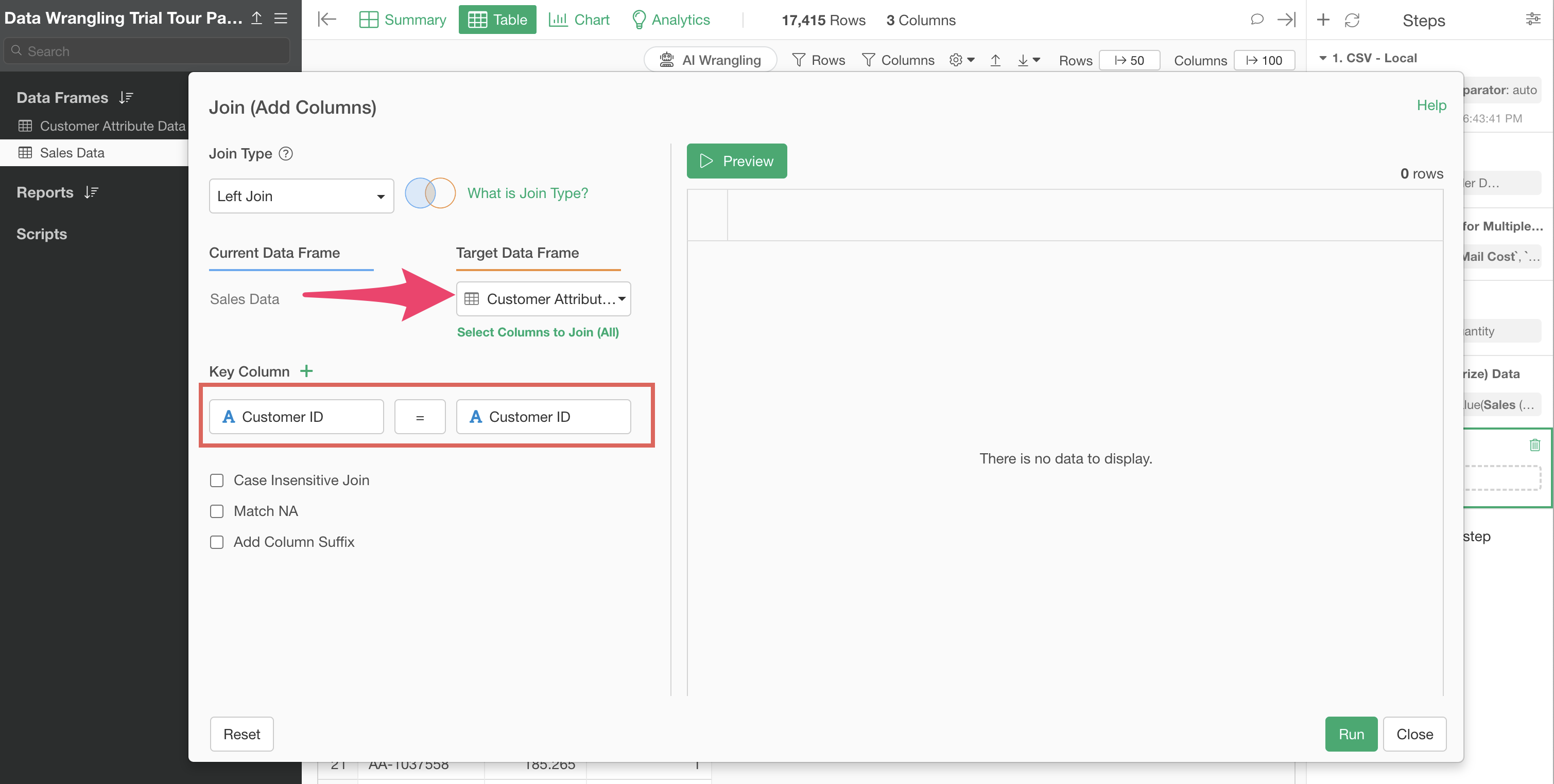
When the Join dialog appears, select “Customer Attribute Data” for the target dataframe, and “Customer ID” for the key column in both dataframes.
You can check the join result by pressing Preview. Columns added by the join are displayed with an orange bar above the column name. If the join looks good, click the “Execute” button.
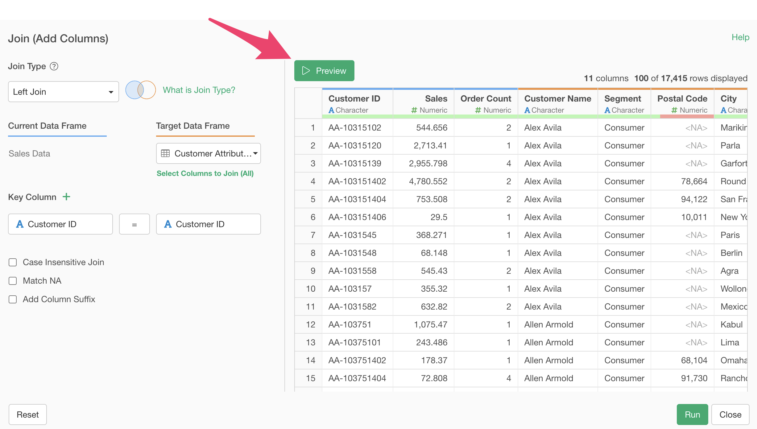
By executing, we’ve successfully added the customer attribute information columns to the customer sales data.
That concludes the Basics of Data Processing part of the Data Wrangling trial tour!
Data Wrangling - Trial Tour
You can check other parts of the Data Wrangling trial tour from the links below. Please try the next part, “Data Structure,” as well.