How to use Correspondence Analysis
Correspondence analysis is one of the frequently used methods for analyzing survey data.
By using correspondence analysis, it is possible to intuitively understand the relationships between questions in surveys that yield categorical responses without an ordinal relationship, as well as the characteristics of the responses.
Required Data Format
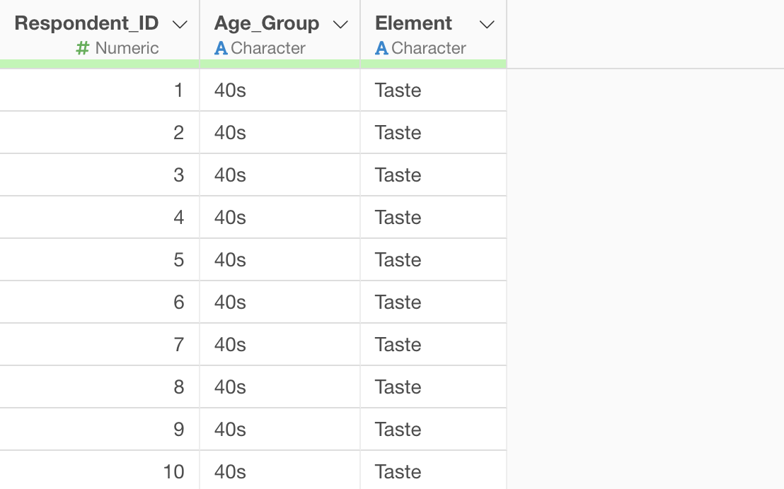
For correspondence analysis, data is required where each row represents one respondent’s evaluation of a single item (e.g., product, service, company). Additionally, only string data types can be selected for variables.
This time, we will use survey data on “what is most important when purchasing beer” as sample data. In this data, each row represents one respondent, and columns include age group and the most important Element.
Performing Correspondence Analysis
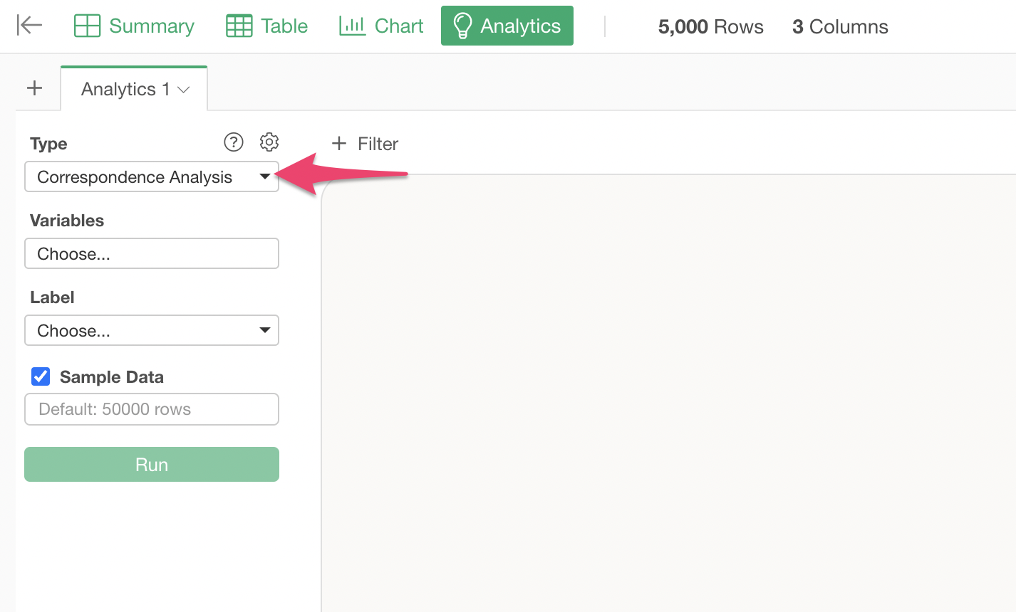
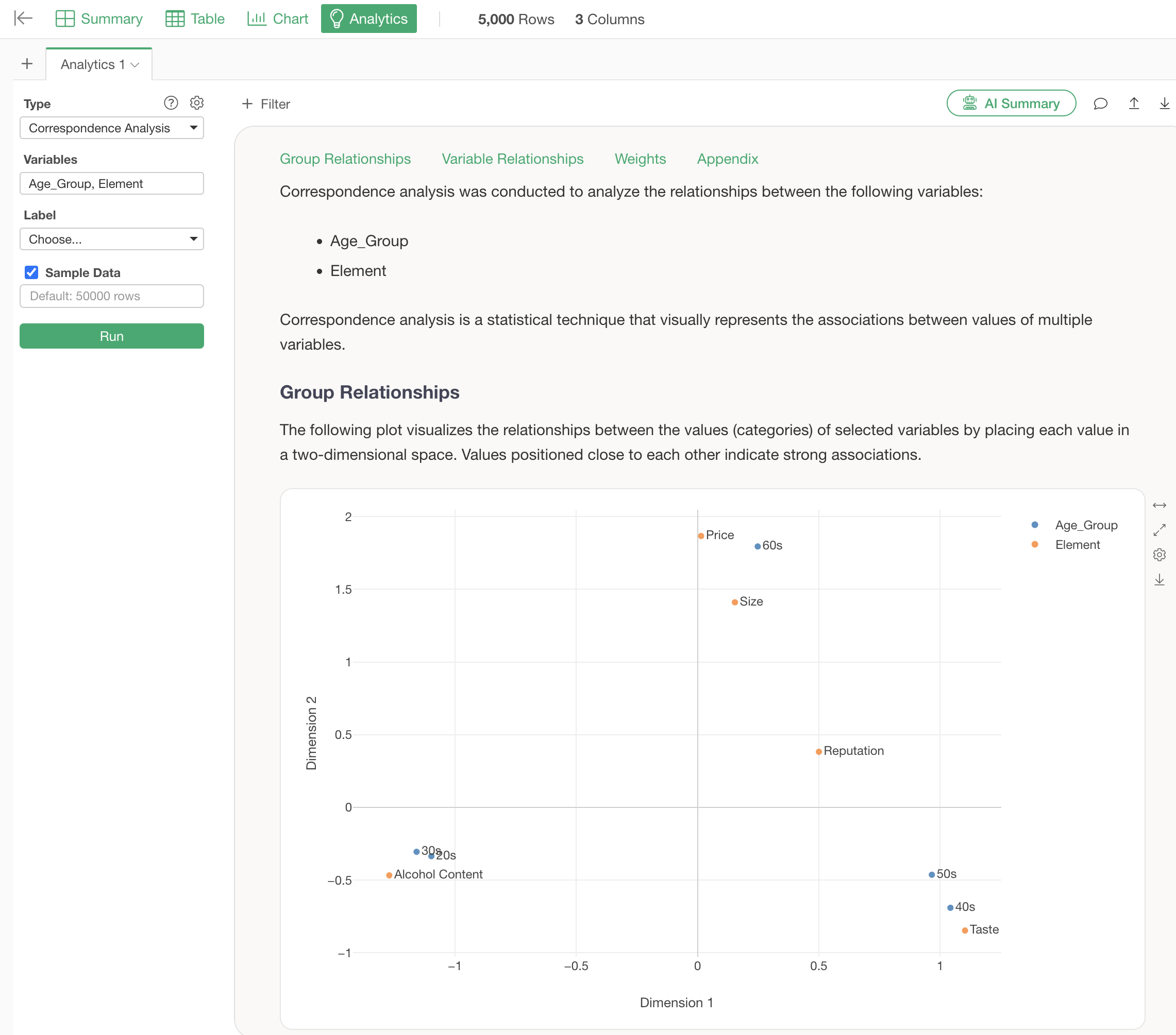
Open the Analytics view and select “Correspondence Analysis” as the type.
Click on the variables columns to select the columns to be used for correspondence analysis. By holding down the Shift key, you can select multiple columns at once.
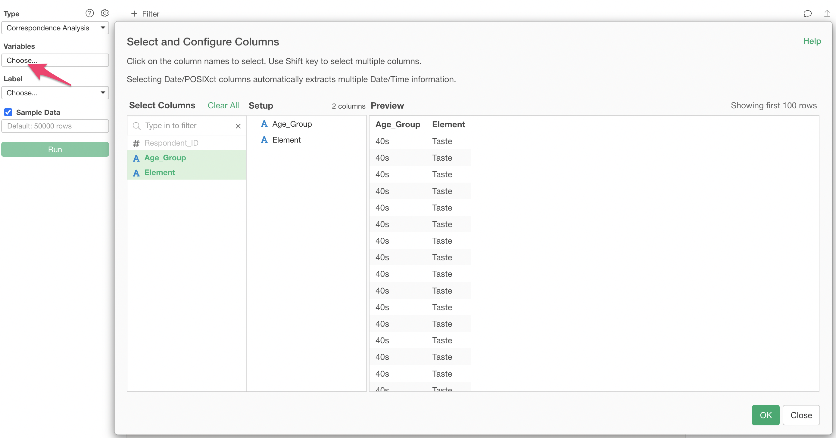
Once the columns are specified, run to display the correspondence analysis results.
Interpretation of Results
Group Relationships
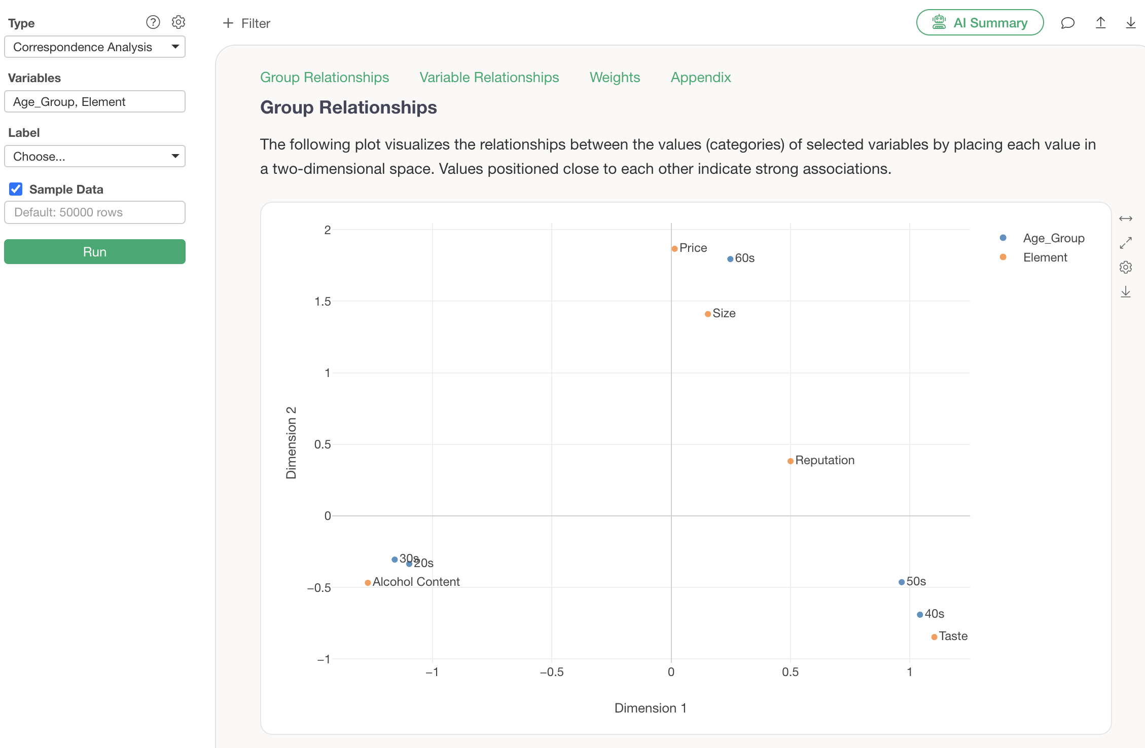
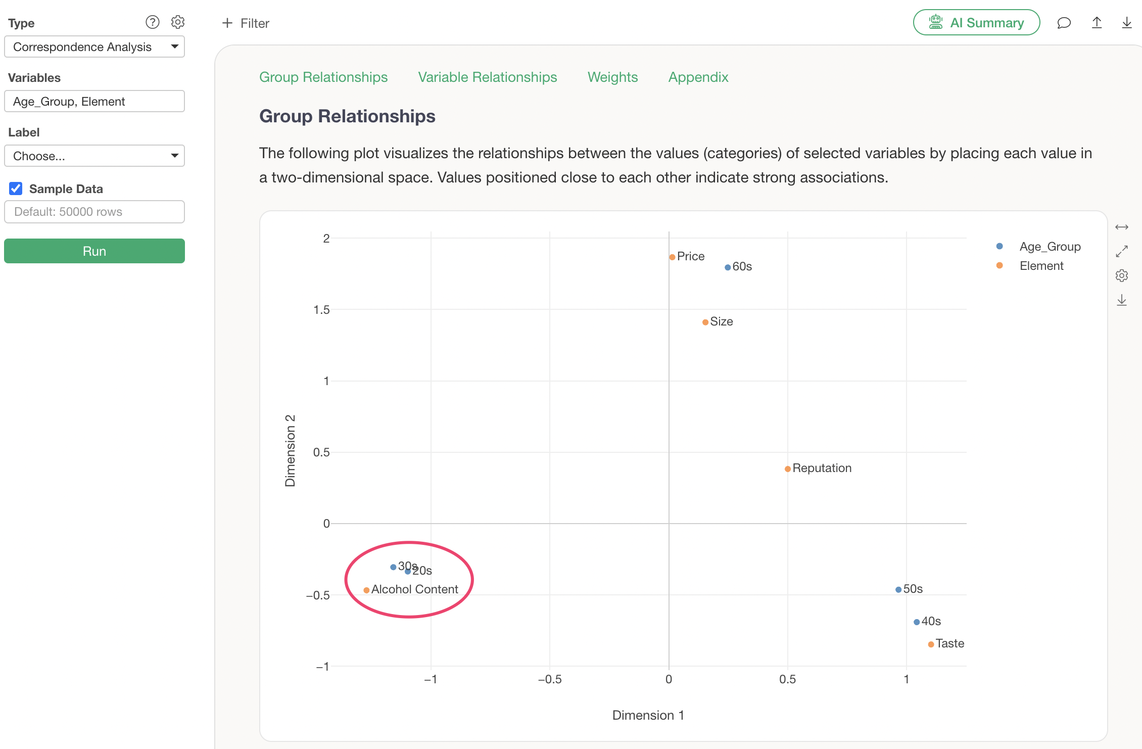
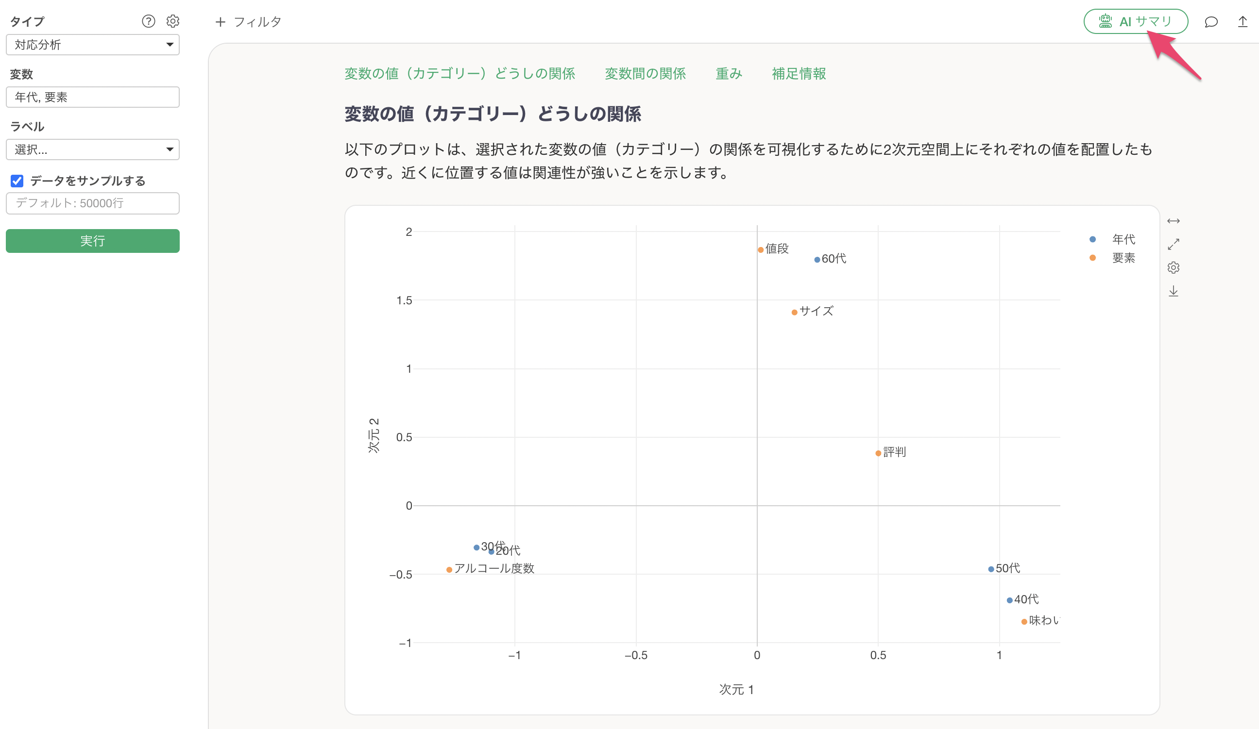
In the section on Group Relationships, a chart visualizing the relationships between categories of each variable is displayed, based on two dimensions (Dimension 1, Dimension 2).
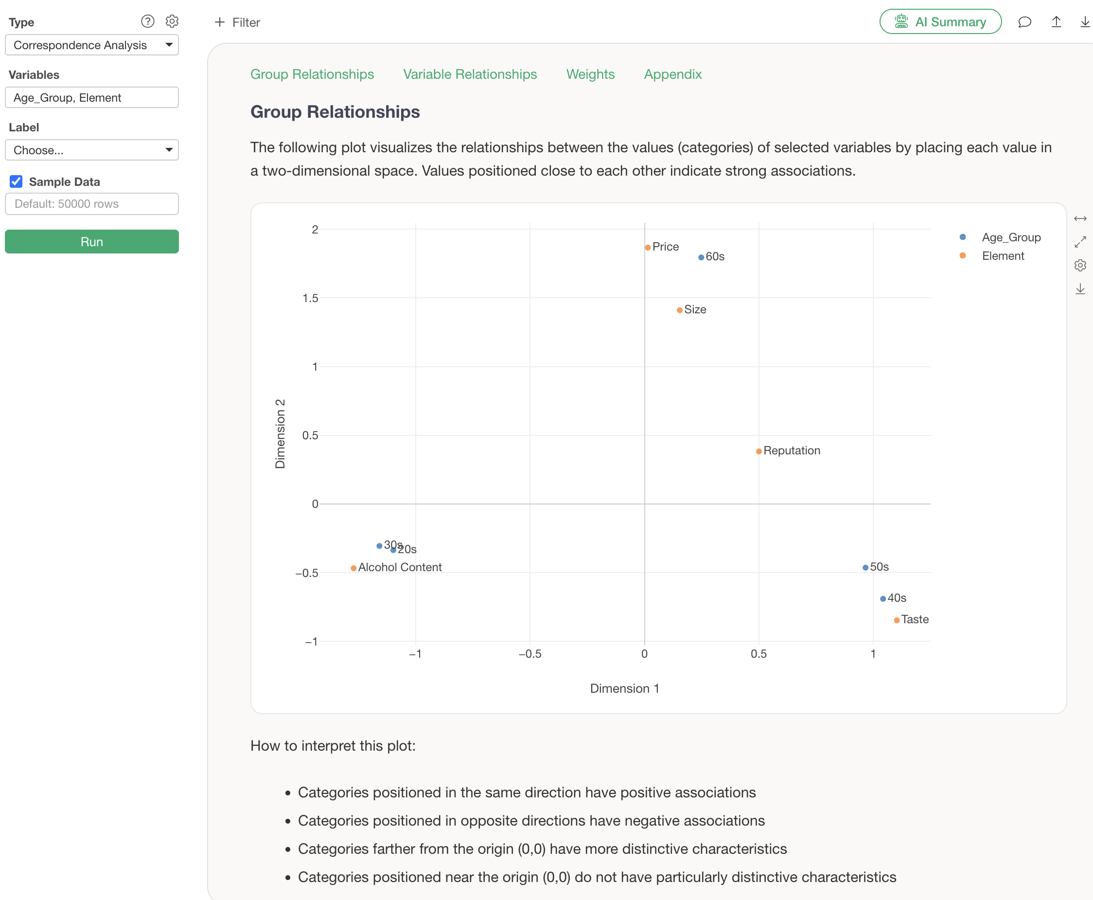
Each point represents a category of a variable, and the colors represent the respective variables (columns).
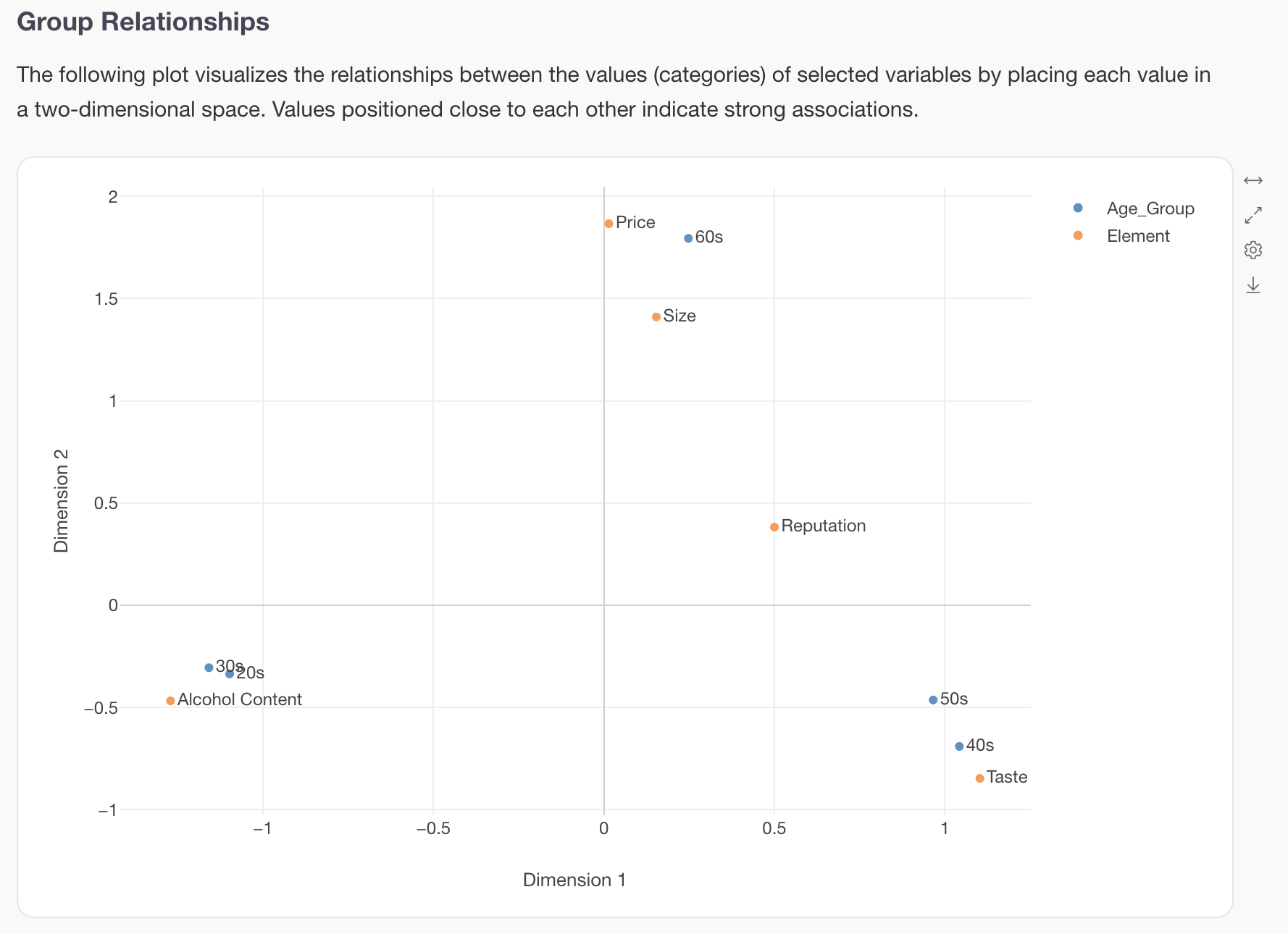
For example, focusing on the blue “Age Group,” it can be seen that the response tendencies of people in their 20s and 30s are similar, thus they are close to each other.
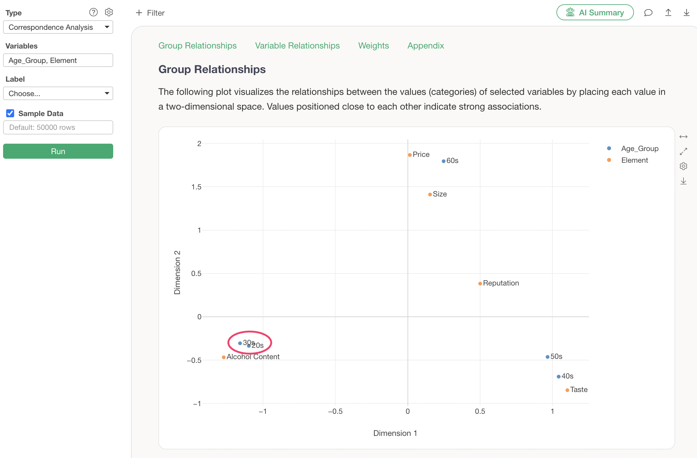
Furthermore, focusing on the relationship between “Age Group” and “Element,” “20s and 30s” are displayed near “Alcohol Content,” indicating that a characteristic of these generations is that they consider “Alcohol Content” important (a large proportion of respondents choose Alcohol Content).
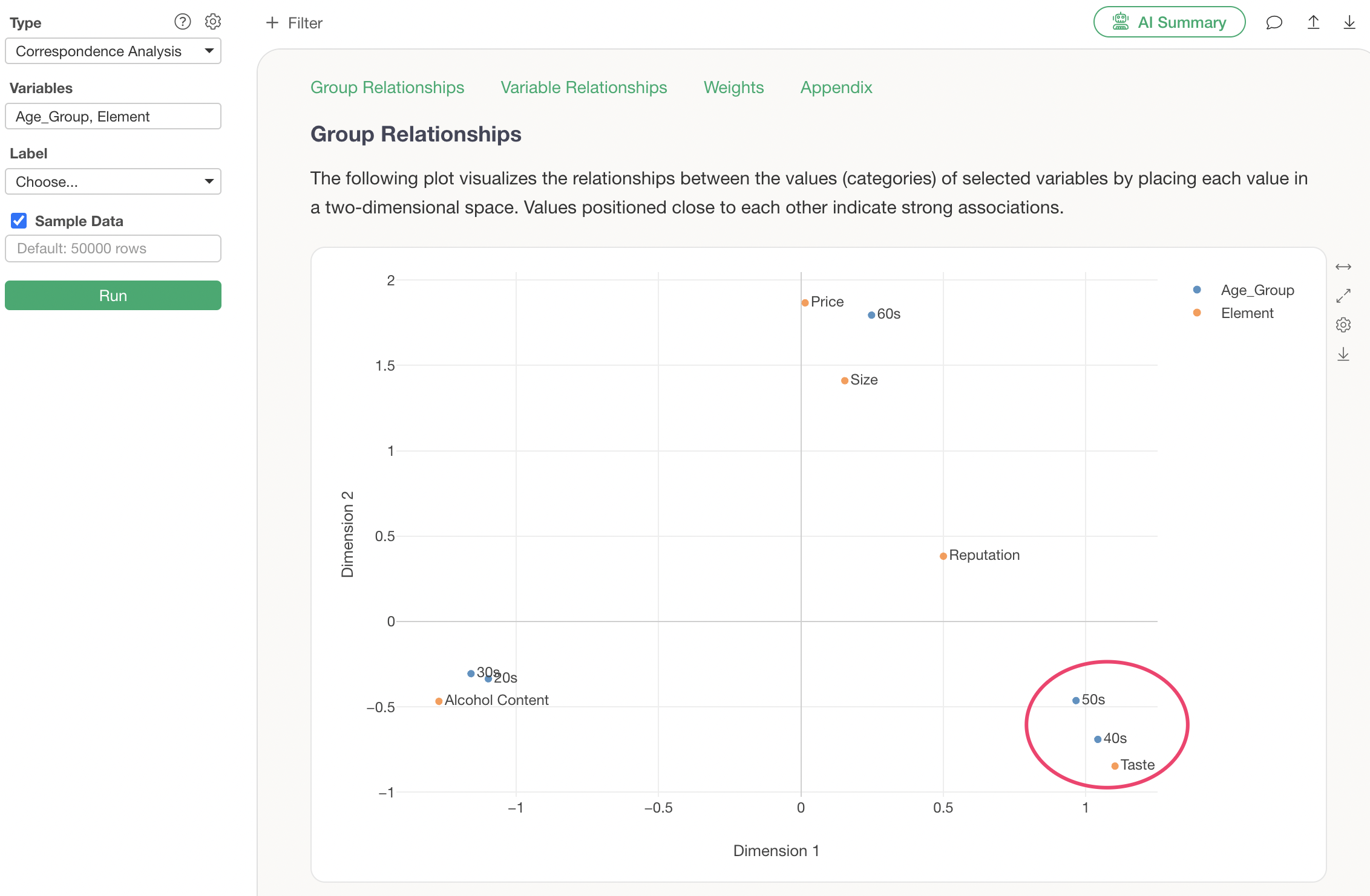
Next, focusing on “40s” and “50s,” their response tendencies are similar, so they are displayed close to each other. A characteristic of these generations is that they consider “Taste” important, hence they are displayed near “Taste.”
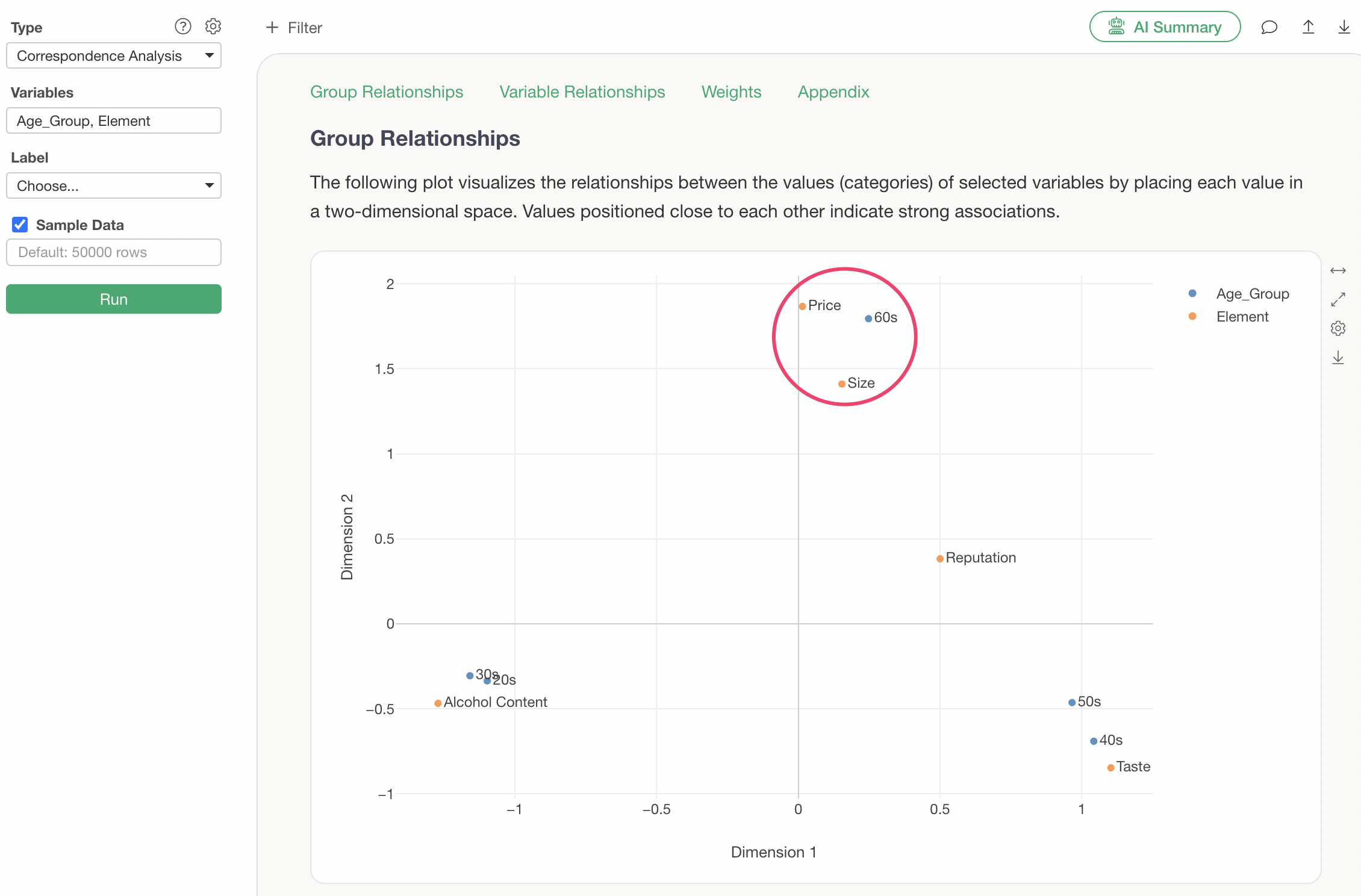
Finally, people in their 60s are displayed separately from other generations because their response tendencies differ. A characteristic of this generation is that they consider “Size” and “Price” important, hence they are displayed nearby.
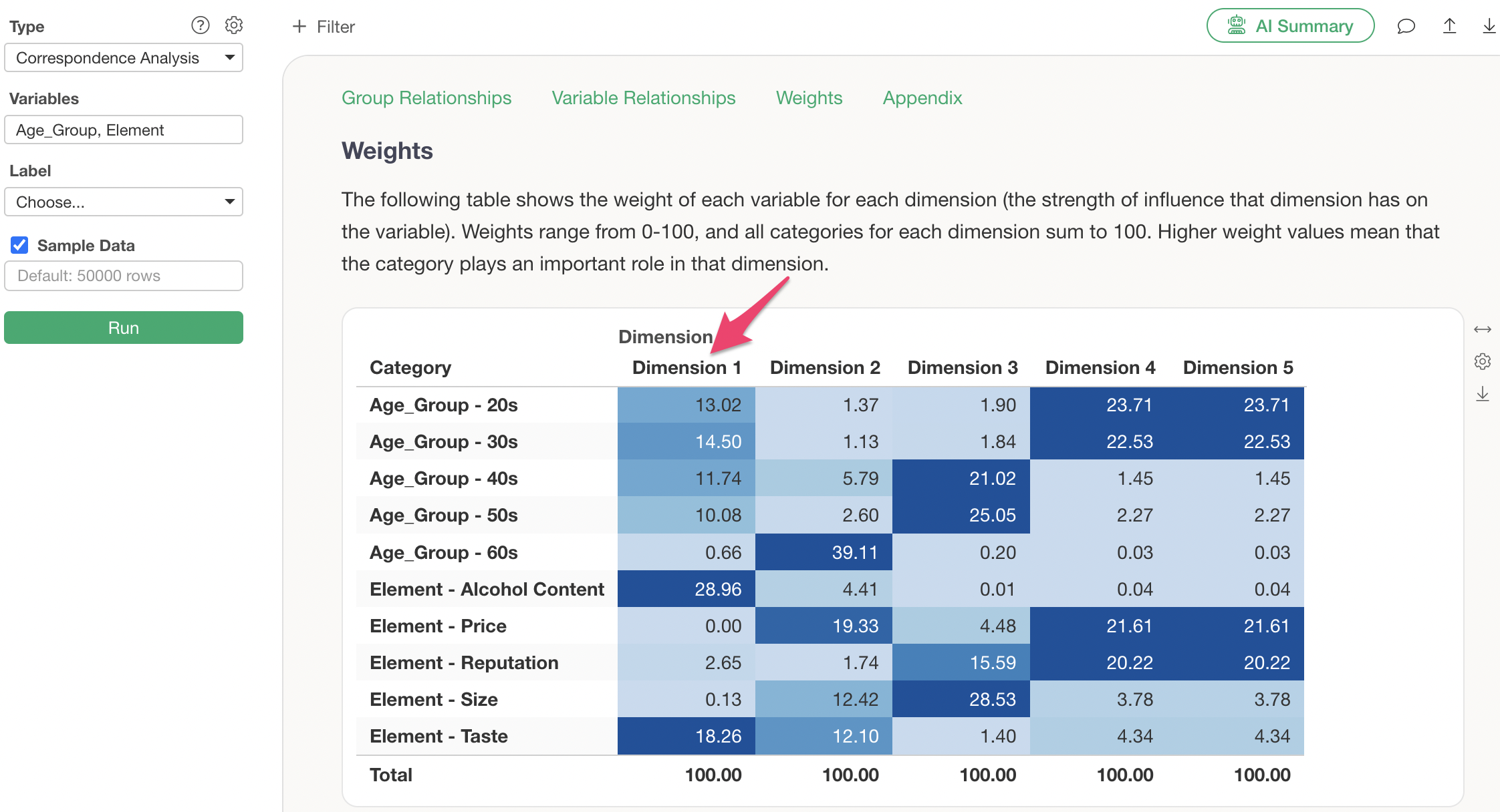
Weights
In the Weights section, the weight of each variable per dimension (the strength of the dimension’s influence on the variable) is displayed. Weights range from 0-100, and the sum of all categories for each dimension is 100.
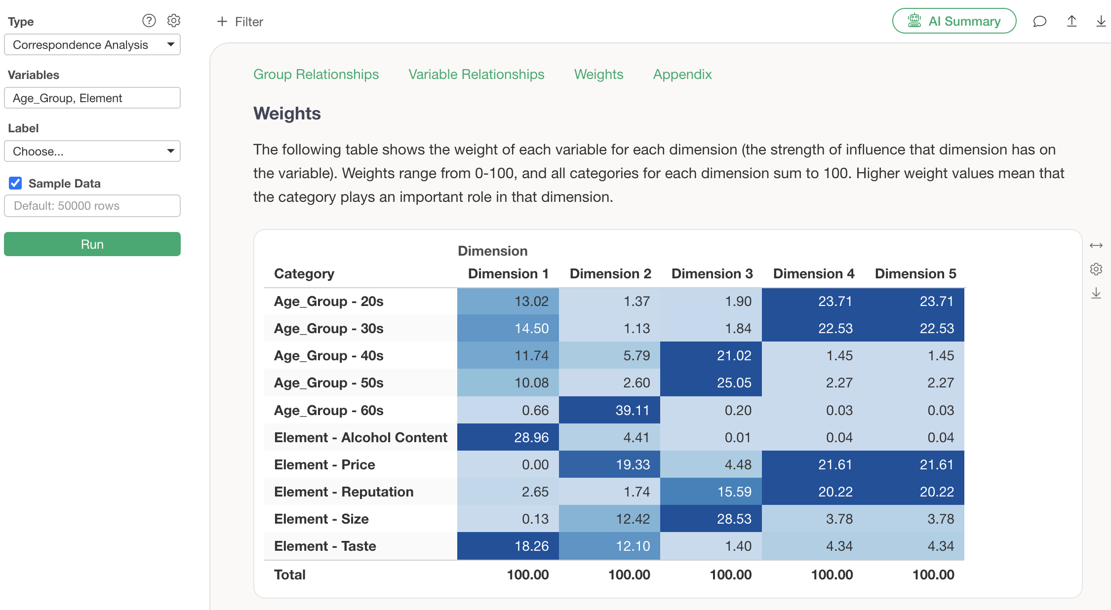
For example, when sorted by Dimension 1, “Alcohol Content” and “Taste” have larger weights, indicating that the characteristics of these categories are well explained by Dimension 1, which is the X-axis.
Contribution Rate
In the Contribution Rate section, you can check how much of the original data’s information (variance) can be represented by the axes created by correspondence analysis.
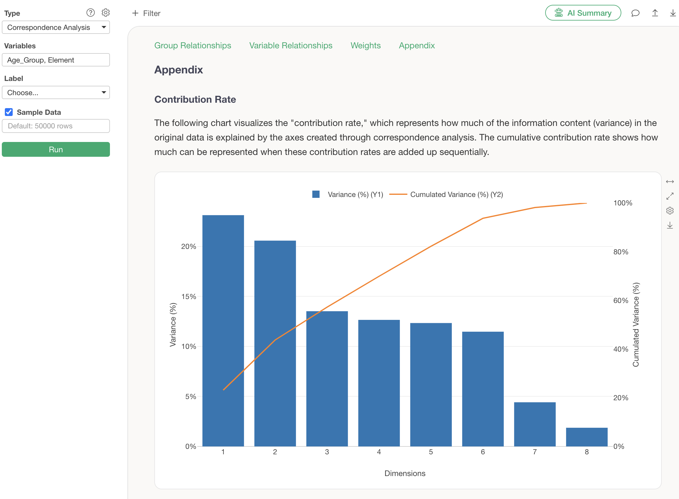
The contribution rate is the proportion of information represented by each dimension, and the cumulative contribution ratio shows how much information is represented when these contribution ratios are summed up.
Summarize Analysis Results Using AI Summary
The AI Summary feature, newly added in v13, automatically summarizes the results of correspondence analysis.
Its usage is surprisingly simple: just click the “AI Summary” button after performing correspondence analysis.
This outputs the results explaining the “relationships between variable values” in correspondence analysis as text.
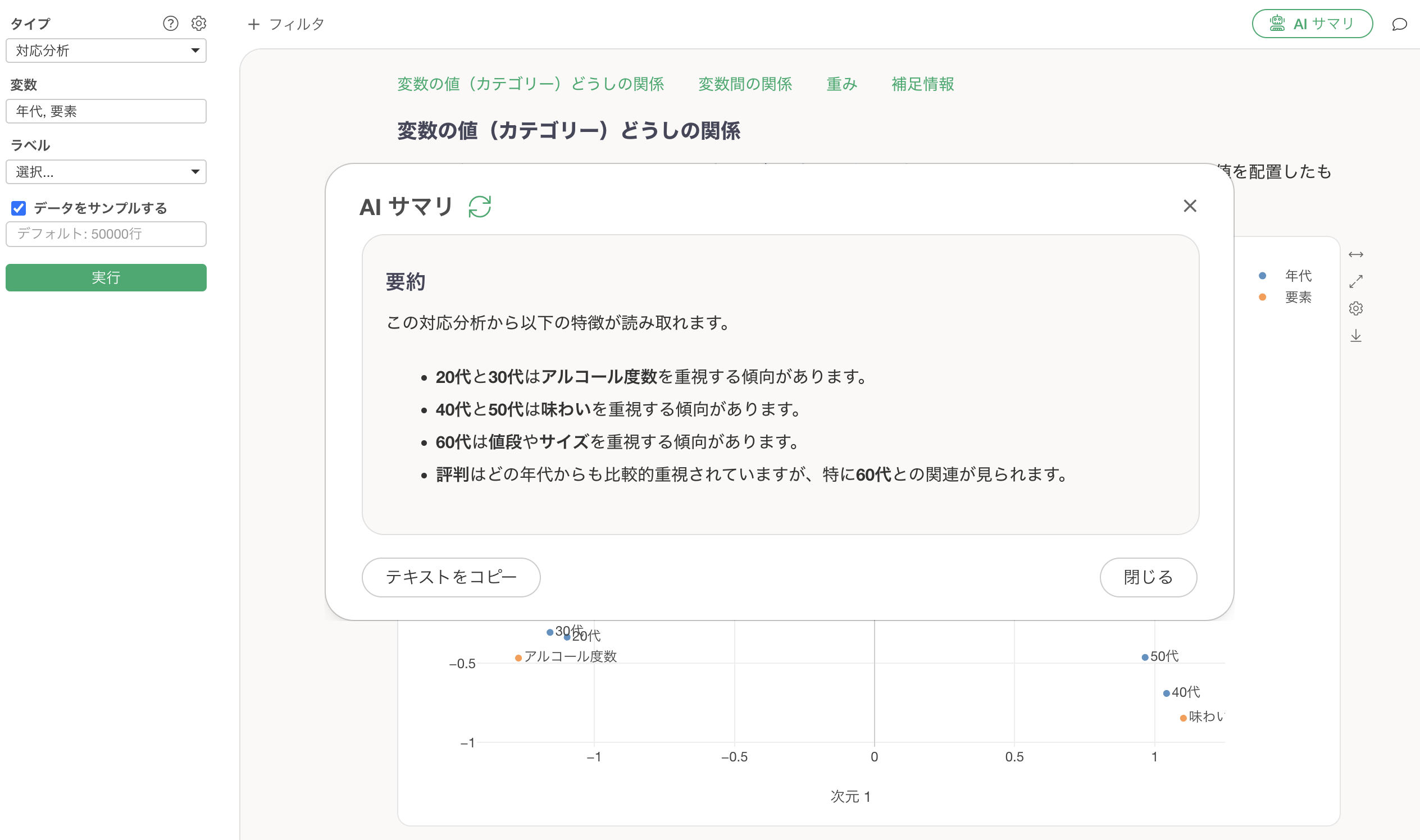
By simply viewing this AI Summary, anyone can easily use correspondence analysis, as the AI determines and informs them of the characteristics without needing to interpret the results themselves.
References
Please refer to the following resources for correspondence analysis.
- Seminar: Introduction to Correspondence Analysis - Link
Frequently Asked Questions about Correspondence Analysis
Here are some frequently asked questions and their answers regarding correspondence analysis.
Q: How are the coordinates for each category displayed in the category tab of Correspondence Analysis calculated?
The coordinates for each category are determined based on the distances between categories. For details, please refer to the online seminar introduced here.