Introduction to Join Part 1 - Adding Columns from Another Data Frame
This is part 1 of ‘Introduction to Join’ series.
- Introduction to Join Part 1 - Bring extra columns from the target - This one
- Introduction to Join Part 2 - Filter data based on another data frame - Link
Sometimes, you might want to add extra columns from another data frame. They might be the detail information of the customers, different metrics about the countries, etc.
You might be familiar with this type of operation as 'VLOOKUP' in Excel and 'Join' in SQL.
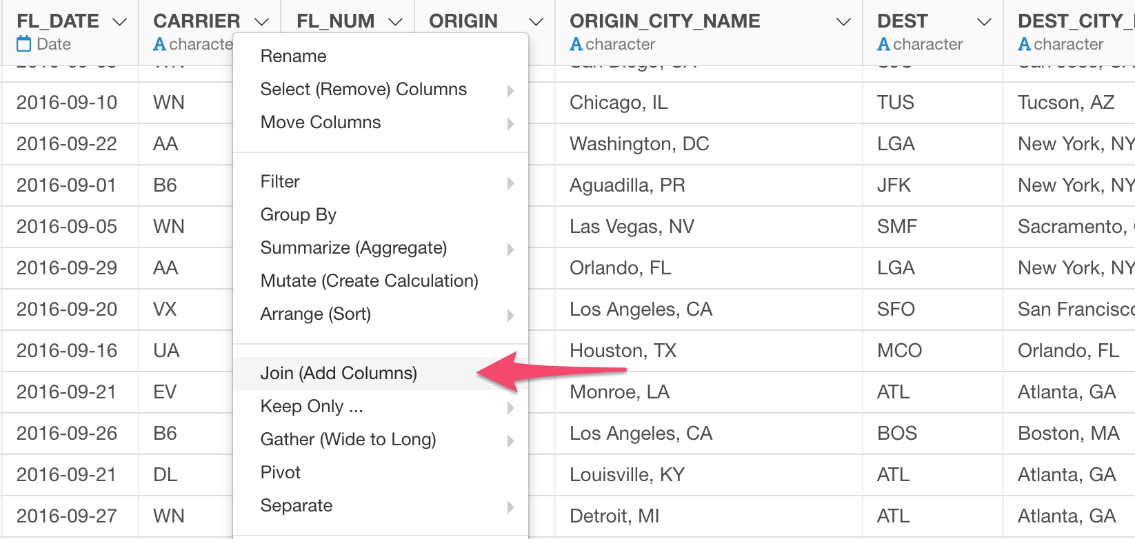
Very similar in Exploratory, there is the 'Join' command, which you can access from the column header menu, you can use for this type of work.
The Join command brings columns from the target data frame.
There are various methods for joining them.
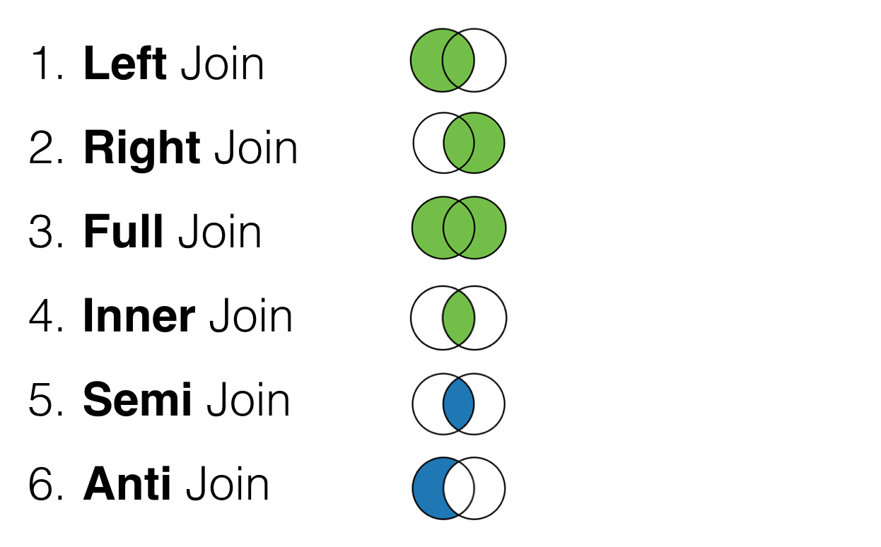
Here is a list of the methods.
And each method will get you a slightly different result.
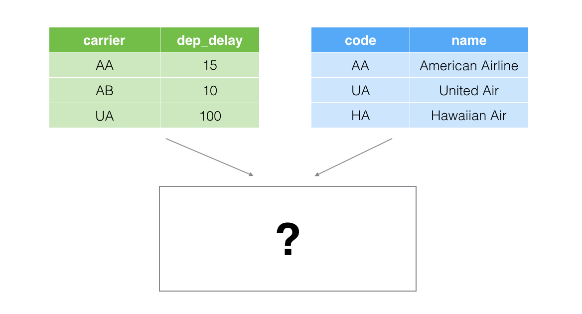
Let's take a look at how each method works first, then we'll look at how it works in Exploratory with examples.
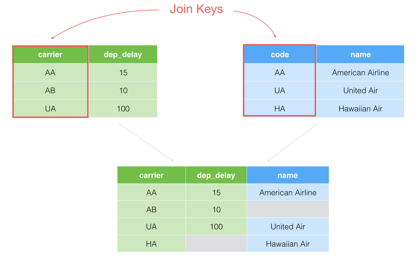
1. Left Join
This is basically the same as ‘VLOOKUP’ if you are familiar with Excel or ‘Left Outer Join’ verb if you are familiar with SQL.
'Left Join' method keeps all the rows from the current data frame and set NAs for the rows that don't have any corresponding data in the target data frame.
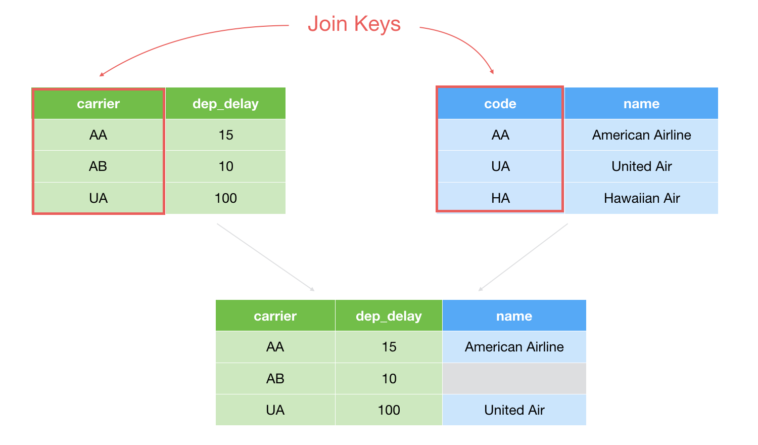
The green table is the current data frame you are working on and the blue is the Target data frame that you want to join to.
We want to use 'carrier' column from the source data frame and 'code' column from the target data frame as join key columns to match, and we want to bring 'name' column from the target data frame.
You can see that 'AA' (the 1st row) exist in both the current data frame (the left side) and the target data frame (the right side), hence we'll have 'AA' row in the result. And same as 'UA'.
However, the 'AB' in the 2nd row doesn't have any corresponding value in the target data frame, hence it doesn't have any value for the 'name' column in the result.
2. Right Join
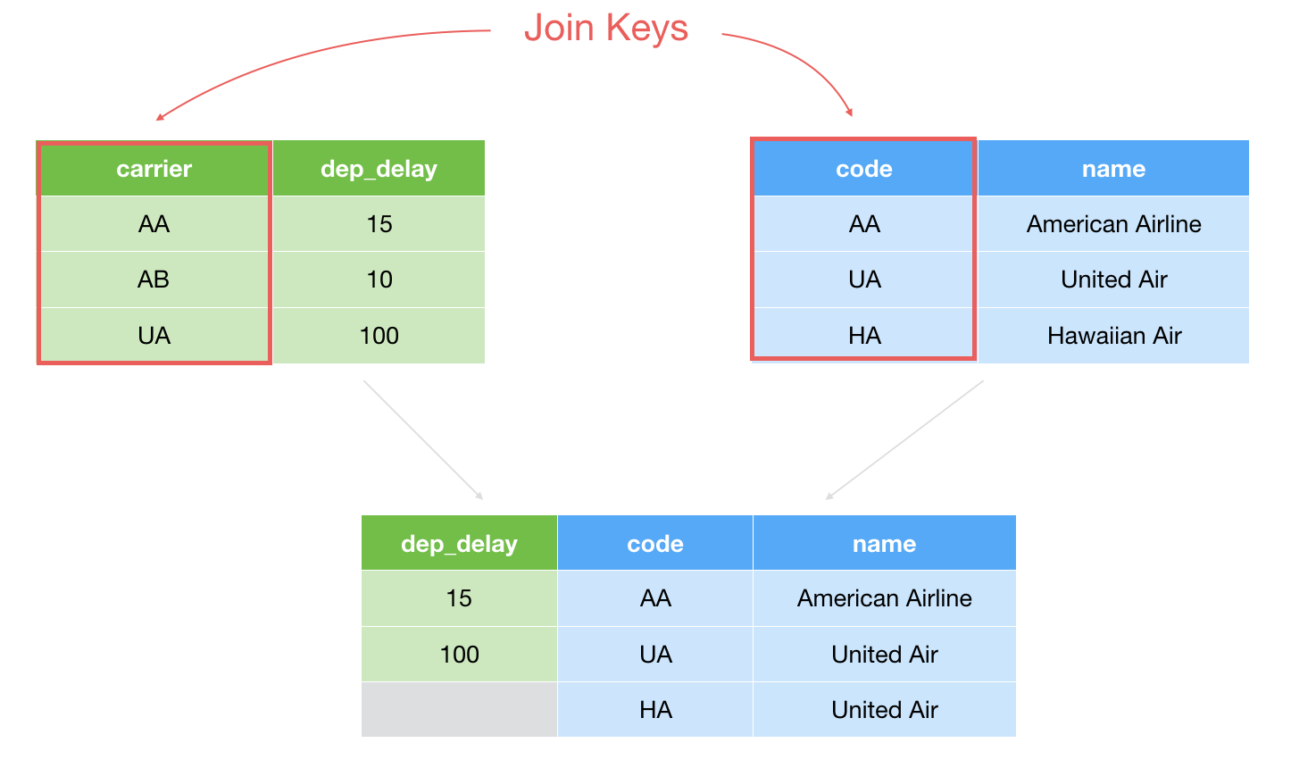
The Right Join is basically the opposite of the Left Join in terms of how to handle the non-matching rows. It will keep all the rows of the target data frame and set NAs for the rows that don't have any matching in the current data frame.
Note that the rows from the current data frame, which don't have any corresponding values in the target data frame will be removed from the result data frame.
3. Full Join
This is essentially a combination of Left Join and Right Join. It will keep all the rows from both the current data frame and the target data frame and set NAs for the rows that don't have any corresponding values.
4. Inner Join
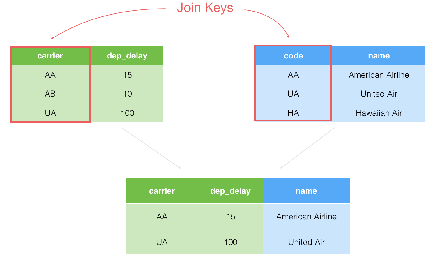
This is sort of the opposite of the Full Join. It will keep only the rows that have the corresponding values in both data frames.
Example
Sample Data
If you are interested in trying out by your hands you can download the following two data sets and follow the steps below.
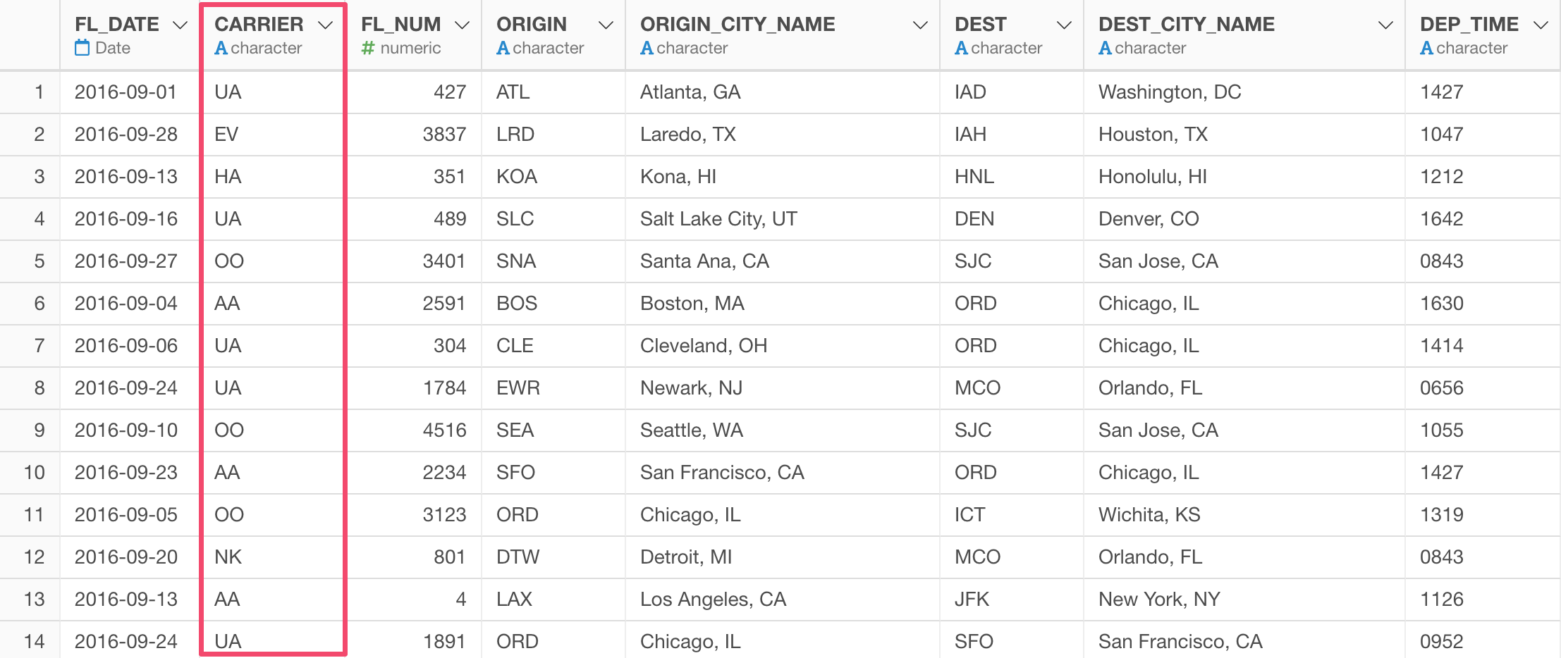
We are going to use this US Flight Delay data for demonstrating how you can use Join command in Exploratory.
Here is how the data looks like.
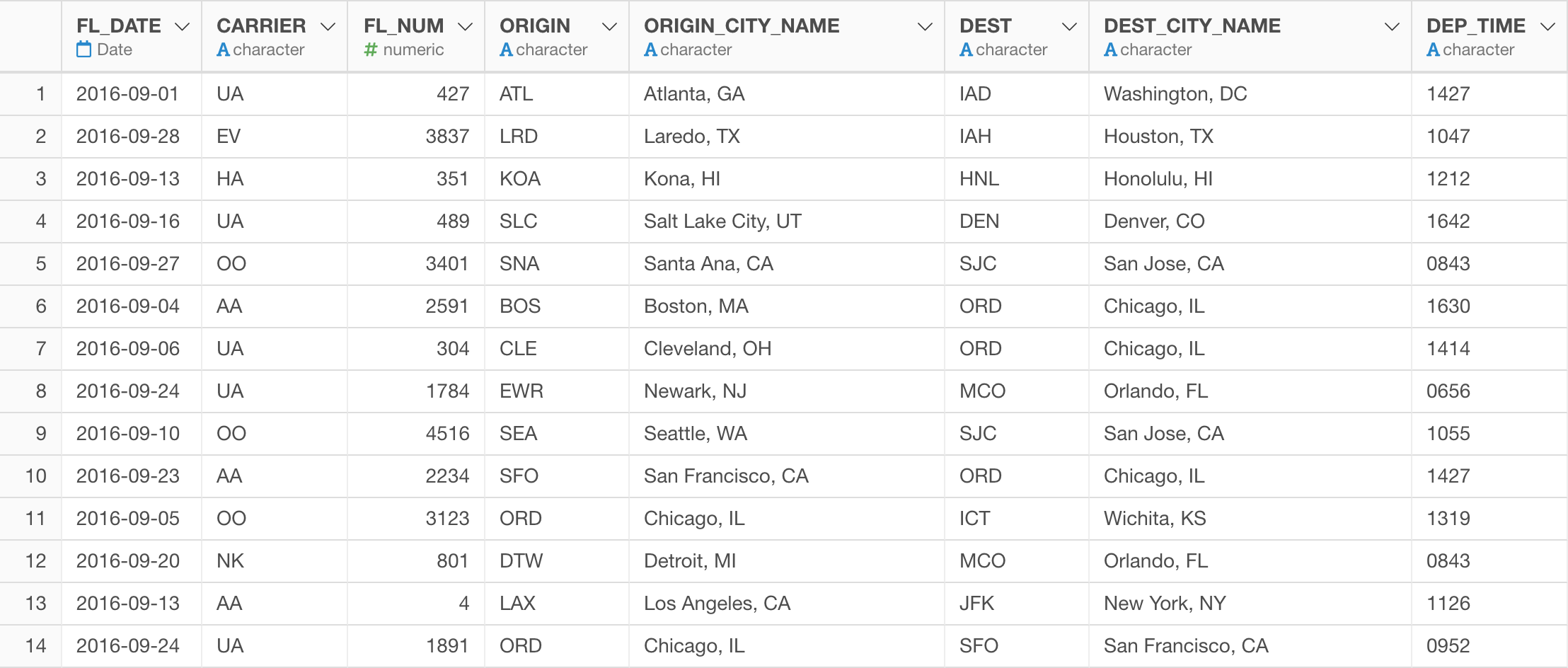
When you look at Carrier column, we are not sure which carrier companies these two letters codes stand for.
Conveniently, we have another data frame called 'carrier_code_list' that has the mapping between the two letter codes and the company names.
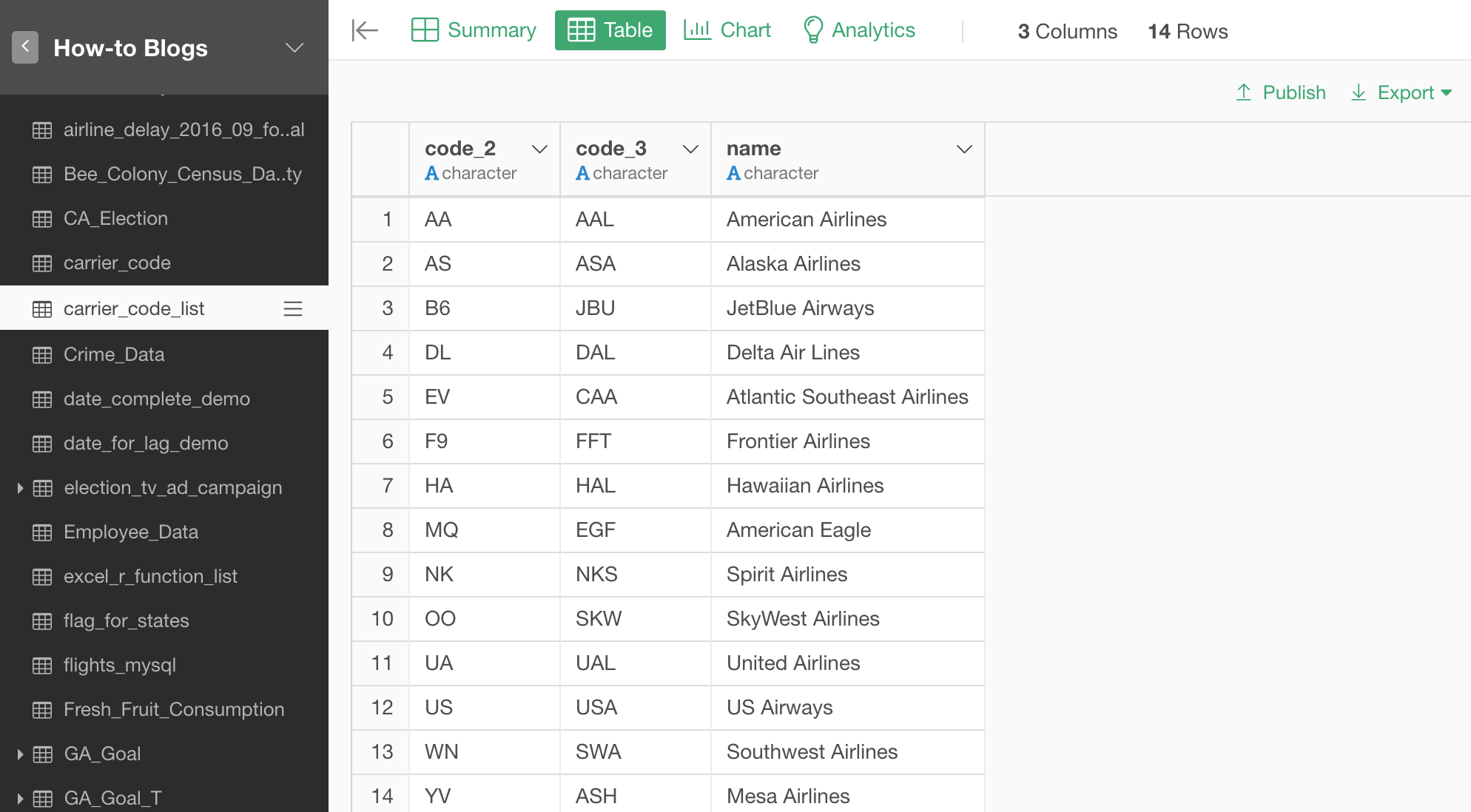
We're going to 'join' this data frame to the 'US Flight Delay' data frame with various join type options.
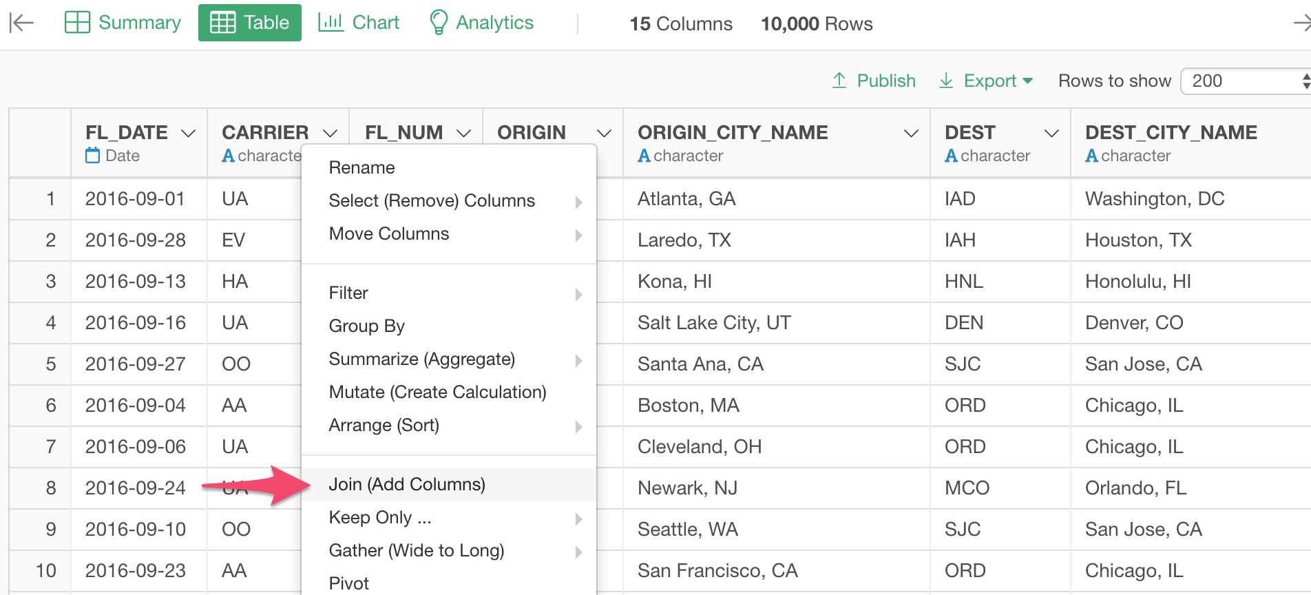
Let’s go back to the US Flight Delay data frame and open the Table view.
Join with Left Join
We'll start with Left Join.
Select 'Join' from the column header menu of 'Carrier' column.
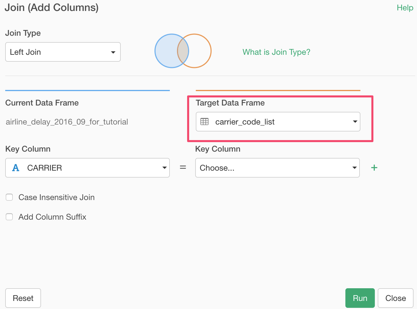
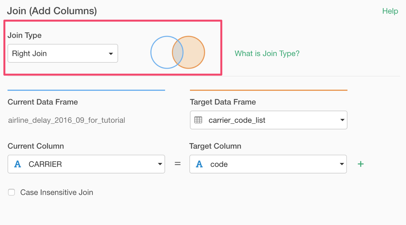
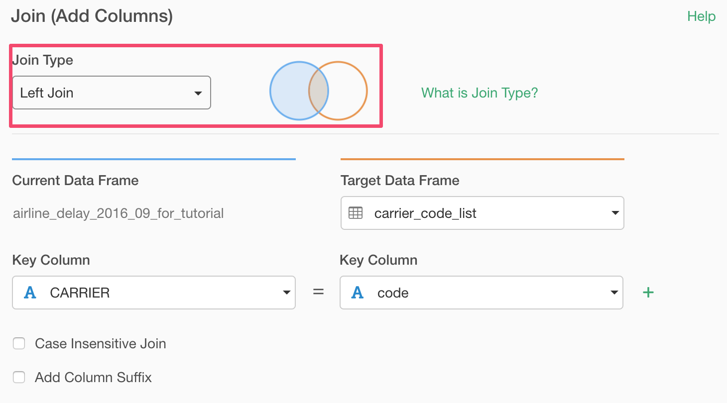
In the opened Join dialog, make sure 'Left Join' is selected because this is the join type we want to use this type.
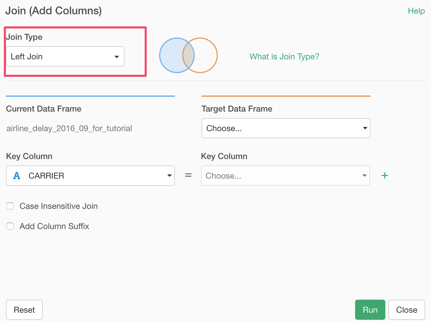
Select the ‘carrier_code_list’ data frame for the 'Target Data Frame'.
And select columns for both Current Data Frame and Target Data Frame. These are the columns that have the 'key' values to match the two data sets.
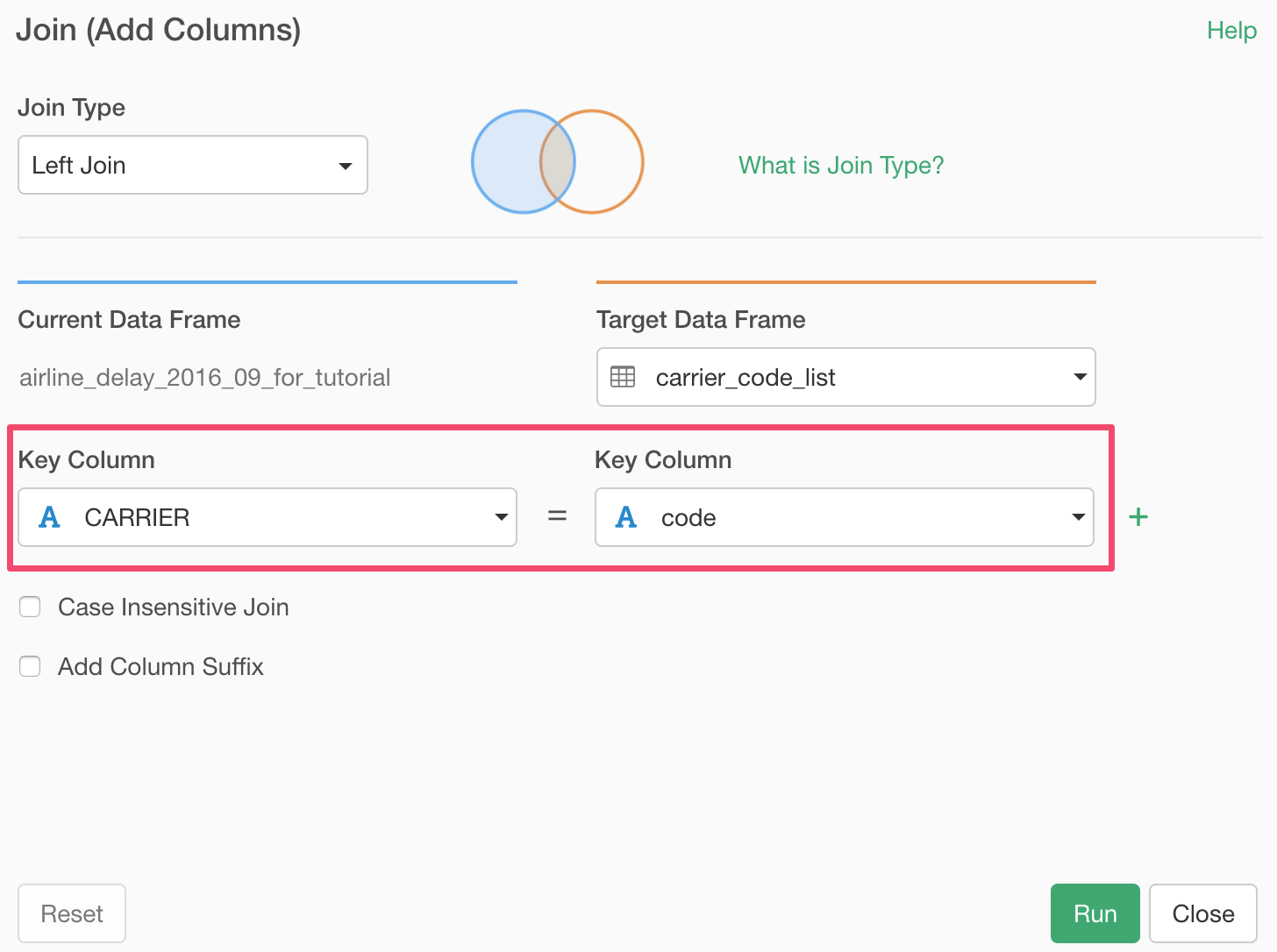
This time, we need only one column (carrier code) to match the two data frames. But sometimes you might need more than one. For example, you might want to use Country and Name to match two data frames.
Once we run the Join command by clicking the Run button, there are two things you'll notice.
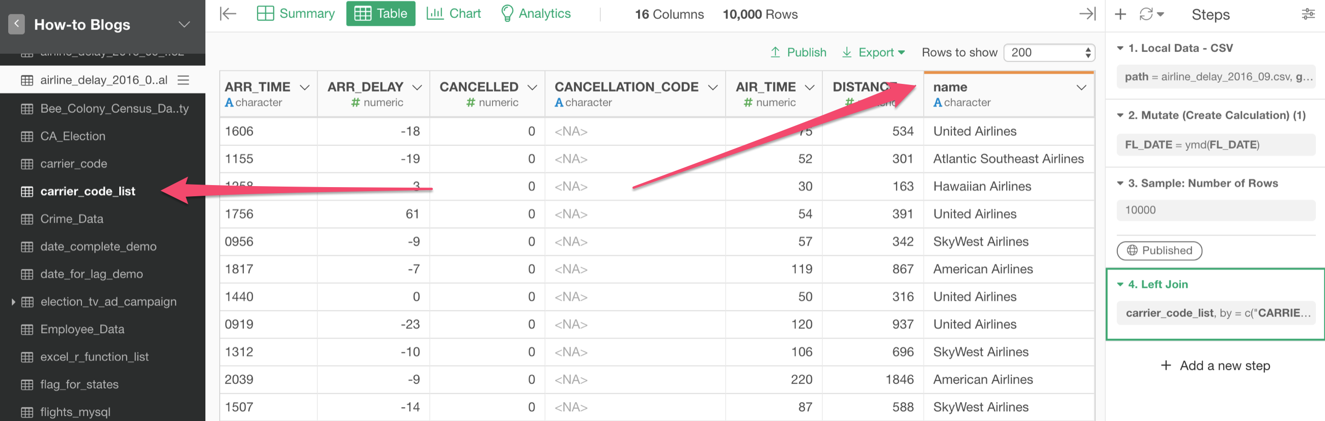
First, you can see the target data frame 'carrier_code_list' is now highlighted at the left hand side.
Second, you can see the new column from the target data frame is added with the orange borderline at the top.
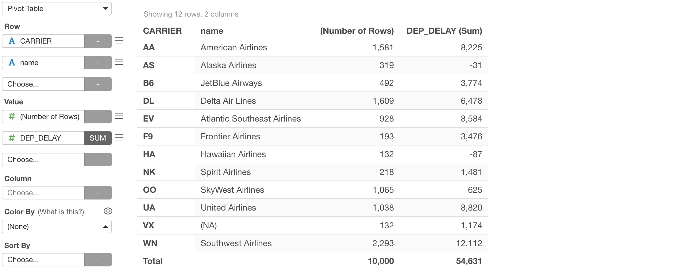
Now, when we go to Summary view, you will notice that there are NAs (missing values) in the 'name' column, which came from the target data frame 'carrier_code_list'.
This means that there are rows from the main data frame that didn’t find the matching values in the target.
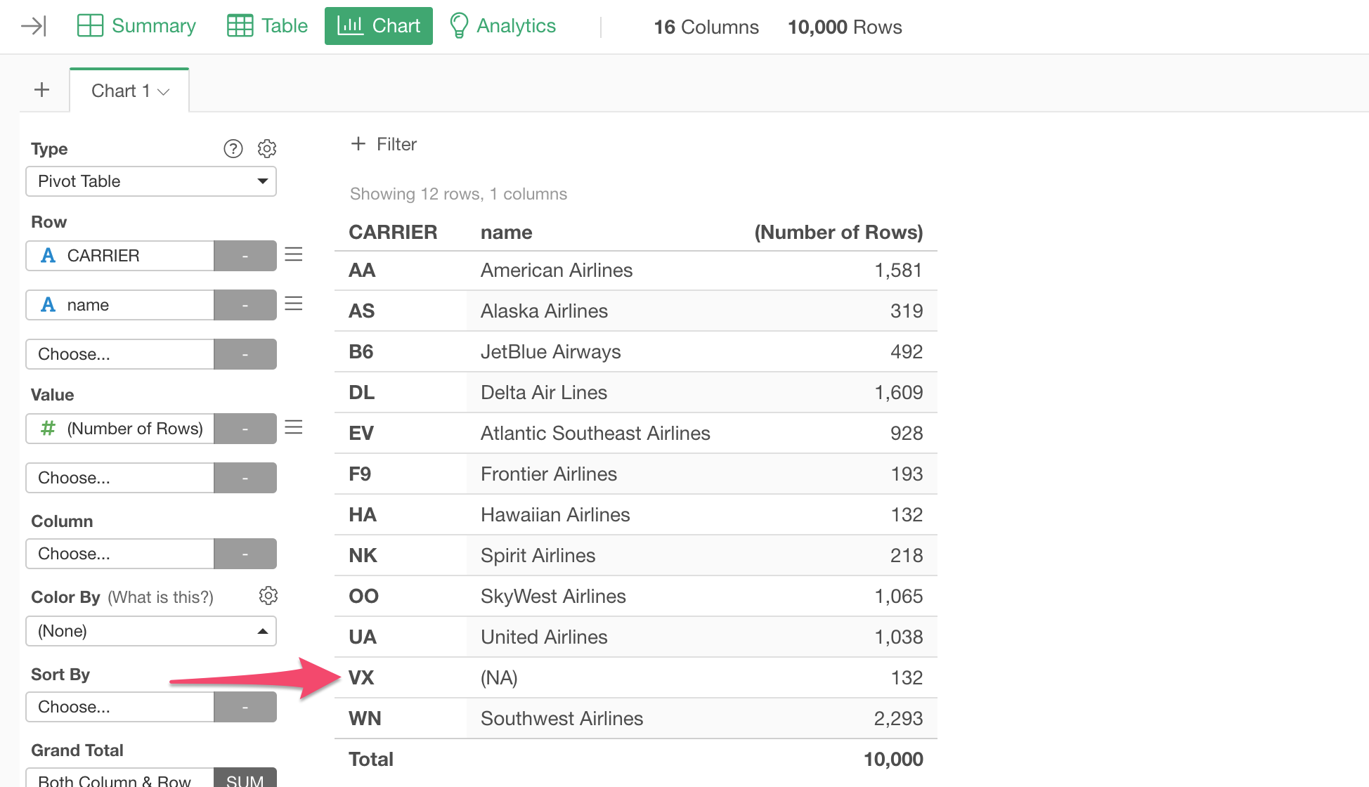
By using the Pivot Table under Chart view, we can see that VX is the carrier that doesn’t have the corresponding name.
Let's see how the other Join types would work.
We can click on the token in the Join step to open the Join dialog and switch between different types quickly.
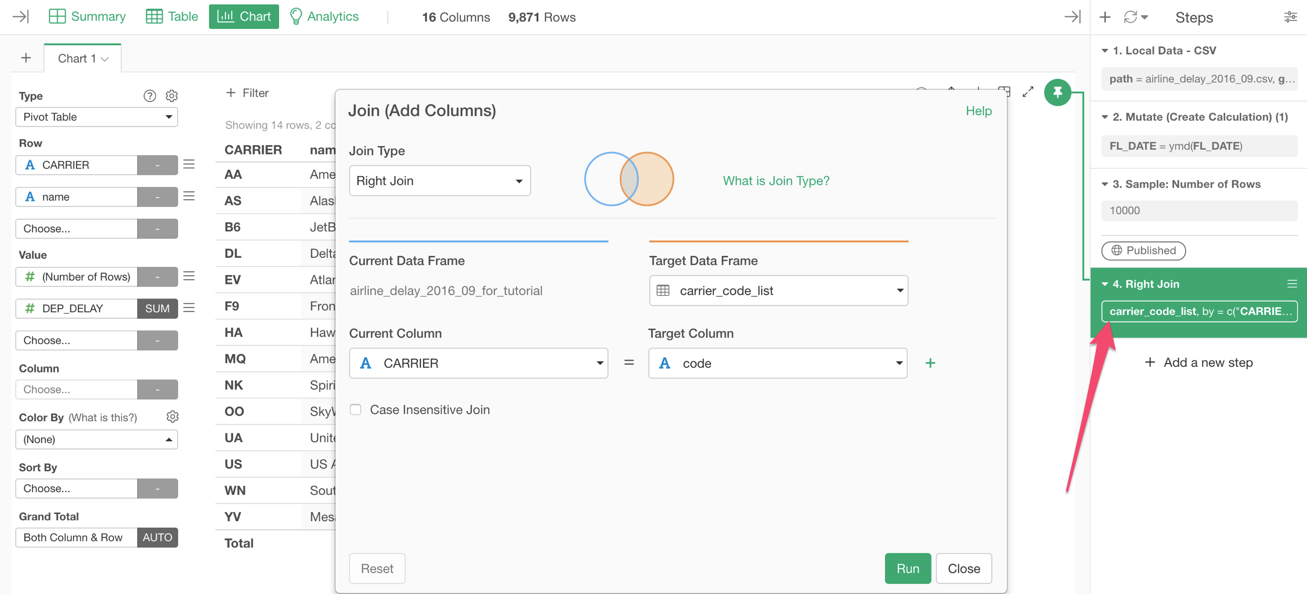
Right Join
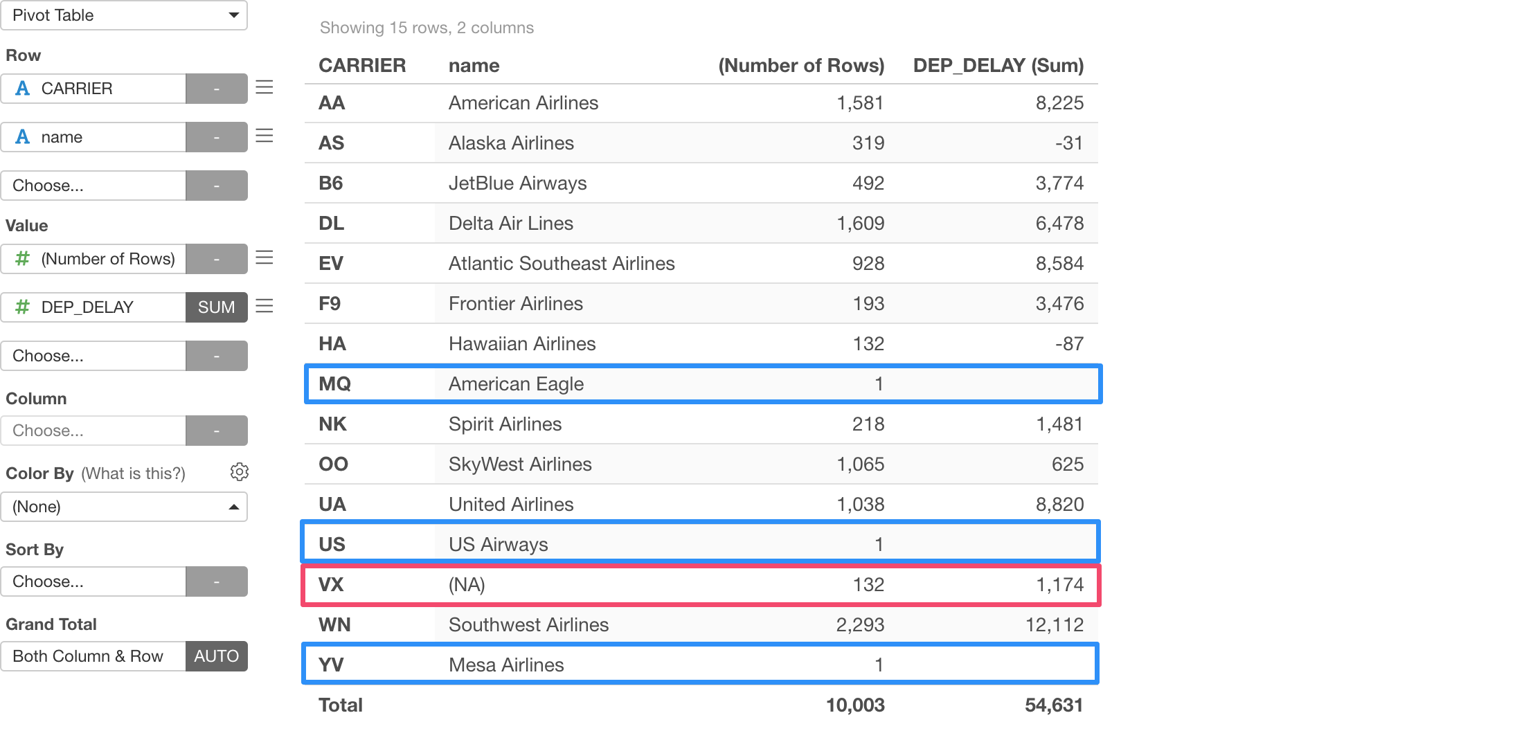
Selecting 'Right Join' and runing the command will now show MQ, US, YV as Carrier in the Pivot Table.
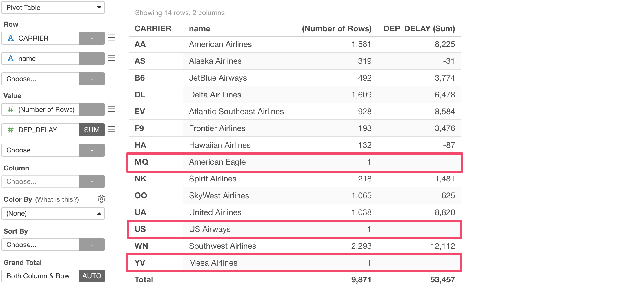
But it indicates that each of those carriers has just 1 row and have no departure delay value.
This is because 'Right Join' keeps all the rows from the target data frame (the right side) even when the current data frame (the left side) doesn't have the corresponding values.
Inner Join
If we switch to Inner Join, the VX, which used to show up with 'Left Join', is no longer showing up and also MQ, US, and YV, which used to show up with 'Right Join', are no longer showing up.
Full Join
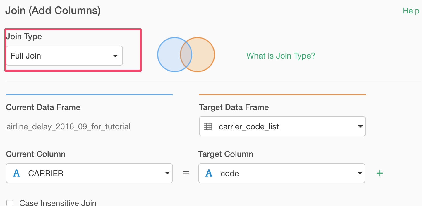
Lastly, we can try Full Join, which would keep all the records from the both data frames.
If you are interested in other types of Join operations, check out the Part 2!
- Introduction to Join Part 2 - Filter data based on another data frame - Link